Inference Engineering · Part 6 of 6
Diffusion, and What Ties It Together
Contents
Every earlier part of this series assumed autoregressive generation: the model writes one token at a time, left to right, and each token depends on all the ones before it. Part 3 showed what enforces that: the causal mask, which is also the only reason the key-value (KV) cache works. This final part looks at another alternative to autoregressive models, called diffusion language models, and then pulls together the thread running through the whole series: the cost of moving bytes.
Diffusion language models have not displaced autoregressive ones, but they are worth understanding because they change the unit of cost. An autoregressive model runs one forward pass per output token, and in decode each pass reads every weight from memory to produce a single token per sequence, as Part 4 showed. A diffusion model starts from a fully masked response and refines every position at once. It runs one forward pass per denoising step, and each step can fill in many tokens. A step costs more than a decode step, but there can be far fewer steps than tokens. The hardware and its memory-bandwidth limit stay the same; what changes is how the work is paid for.
Disclaimer. This post is drafted with assistance from large language models (Claude Opus 5 and DeepSeek V4.1 Flash) based on conversations exploring LLM training and inference. All content has been reviewed, edited, and verified by a human author.
The short version.
- Adding noise needs no model. Diffusion learns the opposite direction, removing noise, one small step at a time.
- Small steps are what make it learnable: undoing a small step has one likely answer, so the model only has to predict a mean.
- For text, noise becomes masking. BERT is a masked diffusion model frozen at a single 15% masking level.
- Diffusion language models pay per denoising step, not per token, and can commit many tokens per step. They are faster and more steerable, not smarter.
- Across all six parts, one constraint explains most optimizations: moving bytes costs far more than doing arithmetic on them.
The insight
Destroying structure is trivial. Creating it is hard.
Adding a small amount of noise to a photo needs no model: just sample Gaussians and add them. Repeat that a thousand times and it becomes unrecognizable: what is left is pure random noise, like the speckle on an untuned TV. Going from photo to noise costs nothing: no model, no training.
The hard direction is the opposite one, from noise back to a photo, and that is the one a diffusion model learns. The trick is to learn it in small pieces. Each forward step (photo toward noise) adds only a little noise, so undoing one step, removing just that little bit of noise, is a small, local, well-posed problem.
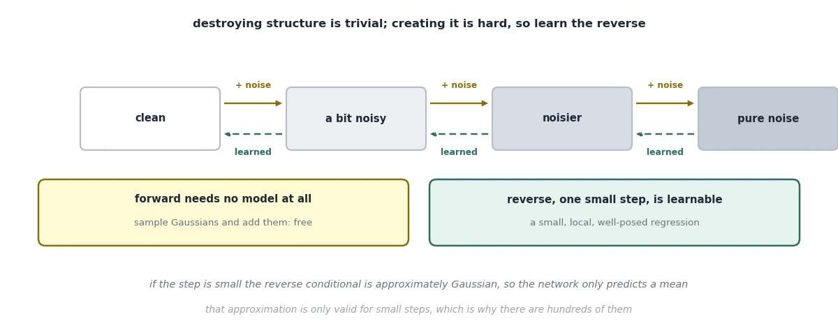 Forward needs no model at all. Reverse, one small step at a time, is a learnable regression problem.
Why the steps must be small
A Gaussian is the bell curve: values cluster around a center (the mean), and the variance sets how spread out they are. Gaussian noise nudges every pixel by a random amount drawn from that curve: usually a small nudge, occasionally a larger one.
At each step, the model answers one question: given the image now, x_t, what did the image one step earlier, x_{t-1}, look like? The answer is a spread of possibilities, written p(x_{t-1} | x_t), because more than one earlier image could have led to the current one. The size of the step decides what shape that spread has.
- Small step: only a tiny amount of noise separates the two images, so the earlier one must be very close to the current one. Every plausible answer sits in one small neighborhood, and the spread is a single bell curve: approximately Gaussian. How much noise each step adds is fixed in advance, so the width of that bell is already known. The network only has to predict where its center is, the mean.
- Large step: starting from pure noise, the plausible answers are a cat, a car, a face: separate clusters with nothing sensible between them. That spread has many peaks, and no single bell curve can describe it. A predicted center would land between the peaks, on a blurry mix of a cat and a car that is not a real image.
The same effect is easy to see in one dimension. Take a “dataset” with only two possible values, -1 and +1: a stand-in for “cat” and “car”. Pick one, add random noise, look at the result, and ask which value it started from.
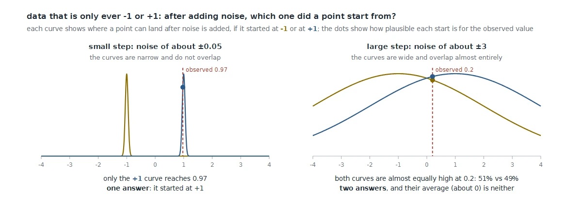 Small noise leaves one plausible starting point. Large noise leaves two, and no single guess between them is right.
- Small noise (nudges of about ±0.05), result 0.97. Starting from +1 needs a nudge of -0.03, which is ordinary. Starting from -1 needs a nudge of +1.97, about 40 times the usual size, which is practically impossible. One answer: it started at +1.
- Large noise (nudges of about ±3), result 0.2. Starting from +1 needs a nudge of -0.8; starting from -1 needs +1.2. Both are ordinary at this noise level, so the two are almost equally likely: 51% versus 49%. Two answers, and the single best guess, their average of about 0, is neither -1 nor +1. That is the one-dimensional version of a blurry cat-car.
The bell-curve shortcut only holds for small steps, which is why diffusion uses hundreds or thousands of them instead of one big one.
What the model is really learning
In training, the model is shown a noisy image and asked to predict the noise that was added to it. Predicting the noise rather than the clean image looks arbitrary: they are algebraically interchangeable. But predicting noise is, up to a scale factor, estimating the score: ∇ₓ log p(x), the gradient of the log density. And the score points toward higher density, toward where real data lives.
For every point in the space, the model learns which direction points back toward real data. Sampling is following those arrows from a random starting point.
Three refinements come up often:
| Refinement | What it changes | Why it matters |
|---|---|---|
| DDIM (Denoising Diffusion Implicit Models) | Treats the reverse chain as an ODE (an ordinary differential equation) and solves it deterministically | 20-50 steps instead of 1000 |
| Classifier-free guidance | Trains with the condition (such as the text prompt) randomly dropped, so one model learns both a prompted and an unprompted prediction. At sampling time, the prediction is pushed further in the direction the prompt moves it, by a factor w |
The “guidance scale” slider |
| Latent diffusion | Runs the whole process inside a compressed autoencoder space rather than on pixels | What made Stable Diffusion runnable on a consumer GPU |
Text breaks the setup
Tokens are discrete. There is no “slightly noisy” version of the token cat.
The fix is to redefine corruption: instead of adding noise, replace tokens with a mask. At t = 0 nothing is masked; at t = 1 everything is.
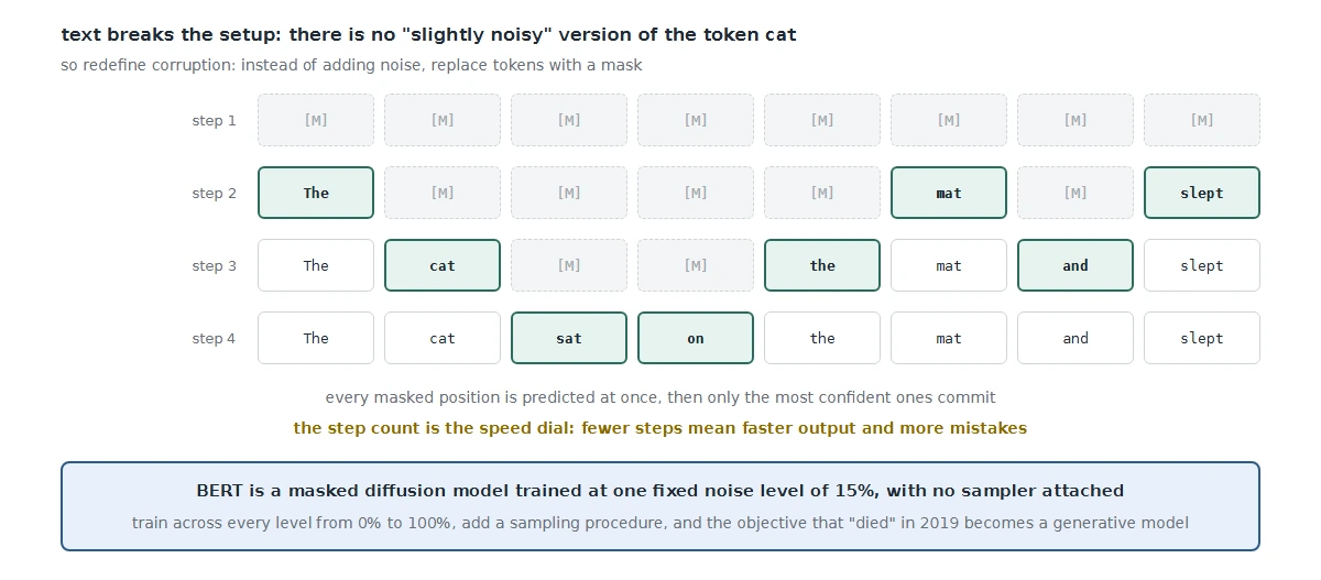 Which connects back to BERT in Part 3.
BERT is a masked diffusion model trained at a single fixed noise level of 15%, with no sampler attached. It only ever learned to fill in a few blanks with most of the sentence visible, so it cannot write from nothing. Two changes turn the same objective into a full generative model. First, train at a random mask level for every example, anywhere from 0% to 100%, so the model also practices on almost entirely hidden text. Second, add a sampler: start from a fully masked response, predict every position, keep the most confident predictions, re-mask the rest, and repeat until nothing is masked. The objective that “died” in 2019 came back as the main alternative to the thing that replaced it, as Part 3 hinted.
Where the quality cost comes from
One assumption does all the damage. Within a single denoising step, every masked position is predicted independently, given only what is currently visible. If two masked slots should read New York, predicting them simultaneously without reference to each other can yield New London.
Committing only the highest-confidence predictions per step is the mitigation: let correlated positions wait until one resolves and can inform the other.
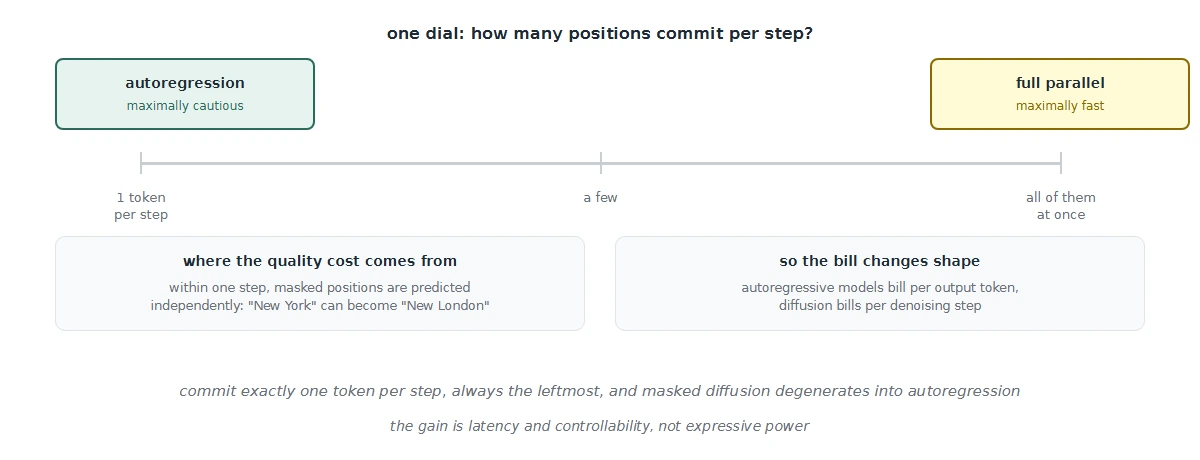 Push the dial to its extreme and masked diffusion degenerates into autoregressive generation.
That framing explains the observed pattern: diffusion wins on short parallel outputs where the independence assumption is cheap, and loses on long chains of dependent reasoning where it is not.
Diffusion is faster and more flexible, not smarter. A diffusion model can fill in positions in any order, while an autoregressive model must go left to right. That sounds like it should let diffusion solve problems autoregressive models cannot, but in principle it does not. Any distribution over text can be written as a left-to-right chain of next-token predictions, and the masked diffusion training objective turns out to be equivalent to training an autoregressive model on every possible generation order at once. With the same model size, data and training compute, the gains are elsewhere: lower latency, because many tokens can be committed per step, and more control, because any position can be fixed, filled in or edited. Switching a serving stack to diffusion should be about speed or steerability, not about better answers.
Side by side
| Autoregressive | Masked diffusion | |
|---|---|---|
| Unit of work | One forward pass per output token | One forward pass per denoising step |
| Tokens per pass | One per sequence | Every masked position is predicted; the confident ones are kept |
| Generation order | Strictly left to right | Any order |
| Attention | Causal: each token sees only earlier tokens | Bidirectional: every position sees the whole sequence |
| KV cache | Yes: the past never changes | Not in the standard form: any position can still change, so each step reprocesses the whole sequence |
| Strong at | Long chains of dependent reasoning | Short outputs, filling in the middle, editing, low latency |
| Weak at | Latency on long outputs, one token at a time | Positions that depend on each other within one step |
What ties it all together
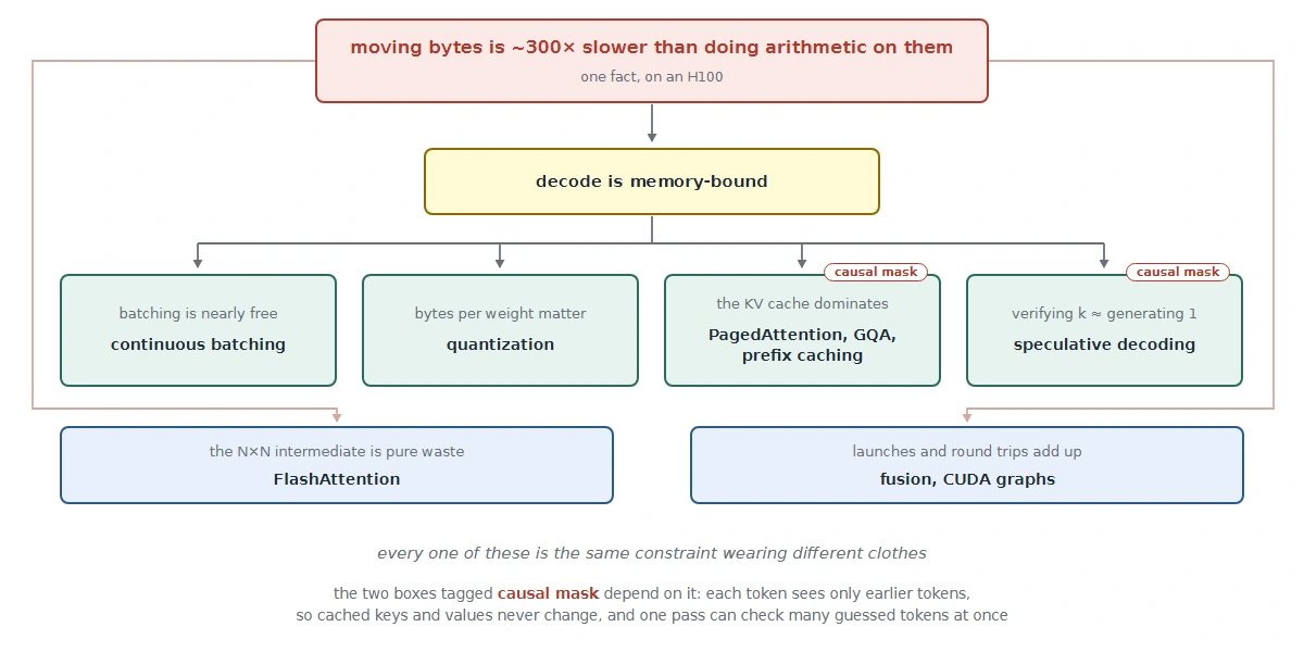
Going back over all six parts, the same constraint keeps surfacing in different costumes.
Every one of these is the same fact wearing different clothes.
A few lessons stand out in hindsight.
The causal mask is load-bearing infrastructure, not just a modeling choice. Decoder-only won partly on training-signal density and format uniformity, but a huge part of it is that causality freezes the past, which is the only reason the KV cache can be built and used, which is the only reason prefix caching and paged blocks and continuous batching are possible at all. One triangular matrix of negative infinity is responsible for the economics of the entire industry.
“Which resource runs out first” is the question behind almost every optimization. Arithmetic intensity versus machine balance is not an exotic GPU thing; it is the same shape as asking whether a query is CPU-bound or I/O-bound. Once the ratio for a kernel can be computed on paper, half the optimization menu reveals itself as a waste of time, and the other half becomes obvious.
Most of the confusions that came up while studying these were category errors, not knowledge gaps. CUDA does not “depend on” kernels; a kernel is what CUDA launches. FlashAttention and PagedAttention are not alternatives; one is a kernel and one is an allocator. ops:byte is not comparing incompatible units; it is a rate over a rate. Decoder-only models do not lack representations; the representation is the thing already eating most of the GPU’s memory.
And the layers exist for different reasons. vLLM depends on PyTorch because rewriting twenty years of array-library work is a bad use of time: llama.cpp proves it is a choice. PyTorch depends on CUDA because NVIDIA opens exactly one door. Those two sentences look similar and describe completely different situations.
If there is one thing to carry out of the series, it is the habit of asking how many bytes does this move, and how much arithmetic does it do with them? before reaching for any optimization. Almost everything else follows.
References
- Philip Kiely, Inference Engineering: Baseten Books, 2026. The series started here.
- Denoising Diffusion Probabilistic Models (Ho et al.): the noise-prediction parameterization.
- Denoising Diffusion Implicit Models (Song et al.): DDIM.
- High-Resolution Image Synthesis with Latent Diffusion Models (Rombach et al.).
- Large Language Diffusion Models (Nie et al.): LLaDA.
- Simple and Effective Masked Diffusion Language Models (Sahoo et al.).
- Your Absorbing Discrete Diffusion Secretly Models the Conditional Distributions of Clean Data (Ou et al.): masked diffusion as an any-order autoregressive model.