Inference Engineering · Part 2 of 6

What Actually Runs the Model

Tisan Das · Sep 27, 2026 · 29 min read

Contents

Part 1 ended with a few hundred gigabytes of weights and an architecture description. This post is about what happens to them next, and it is where the series title starts earning its keep.

The first thing to get straight is that running a model and serving a model are different disciplines.

Running a model means executing one forward pass. Serving means executing thousands of interleaved forward passes per second, over one shared copy of the weights, with per-request state that grows as each conversation grows, under a latency budget.

Running the model can be done with a mere 200-line PyTorch script. However, we need to be efficient to serve the models at scale. That’s what we’re exploring, and the sole purpose of this blog series.

Disclaimer. This post is drafted with assistance from large language models, or LLMs (Claude Opus 5 and DeepSeek V4.1 Flash), based on conversations exploring LLM training and inference. All content has been reviewed, edited, and verified by a human author.

The stack

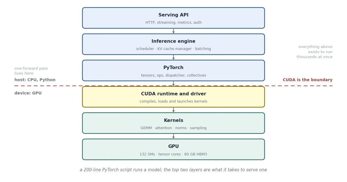The first three layers run on the host CPU (central processing unit) in Python. The bottom two run on the device, the GPU (graphics processing unit). CUDA (Compute Unified Device Architecture) is NVIDIA’s platform for programming its GPUs; an SM (streaming multiprocessor) is one of the GPU’s 132 compute units, and HBM3 is the third generation of its high-bandwidth memory.

What a kernel is, and three meanings of the word

Worth pinning down, because you will hit all three and they are unrelated:

• Linux kernel: the operating system (OS). Relevant here only for the NVIDIA kernel module.
• GPU kernel: a function that runs on the GPU, executed in parallel by thousands of threads. This is the meaning everywhere below.
• Kernel in classical machine learning (ML): convolution filters, the kernel trick. Nothing to do with either.

A GPU kernel is one unit of work you hand to the device. matmul is a kernel. softmax is a kernel. A single decode step of a 70B model launches on the order of a thousand of them.

Each launch costs roughly 3–10 microseconds of CPU-side overhead. That sounds trivial next to a 10–30 ms decode step until you multiply: a thousand launches is 3–10 ms. Many decode kernels finish in only a few microseconds, so the GPU spends that time idle, waiting for the next one. Launch overhead alone can be a double-digit percentage of decode latency. This is the whole reason CUDA graphs exist: record the launch sequence once, then replay it with a single launch.

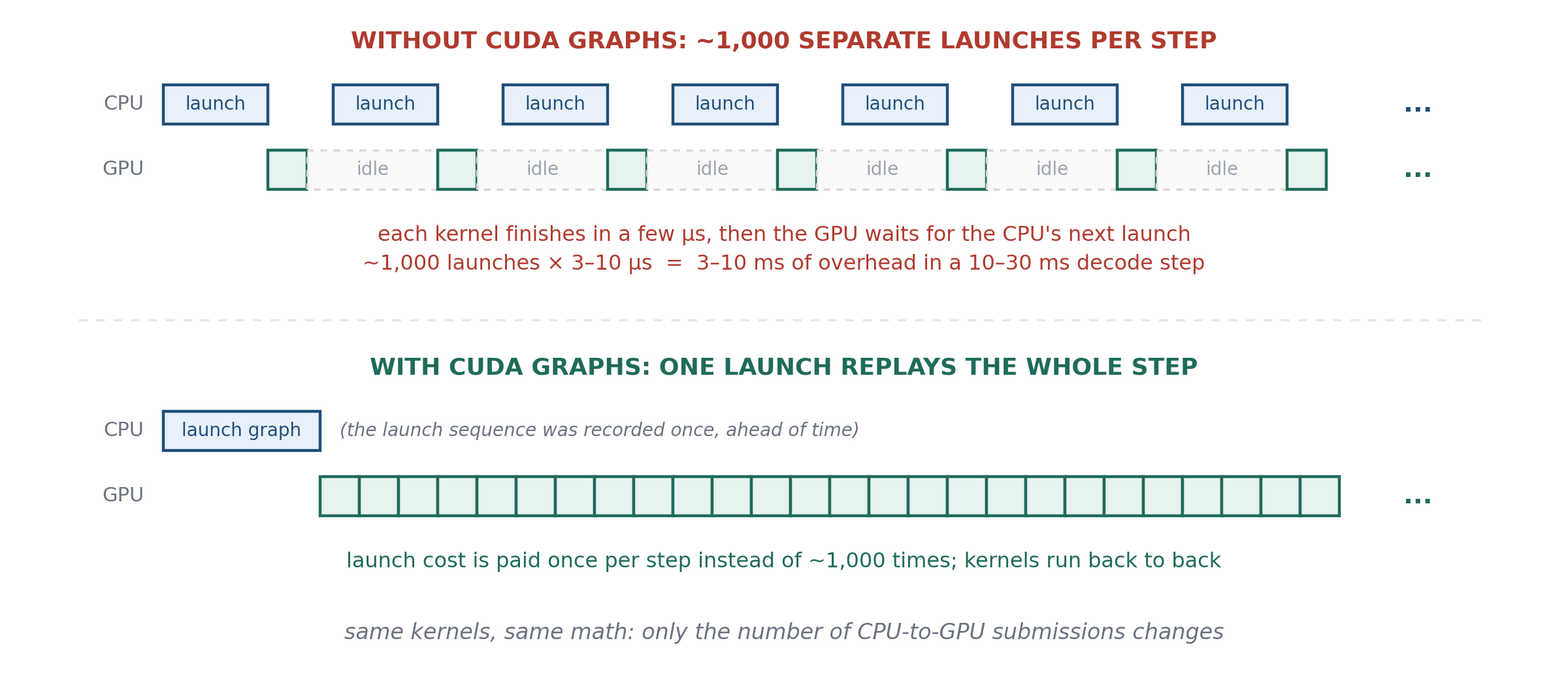
How capture works. During startup, the engine runs a decode step once in capture mode. Instead of running the kernels, CUDA records every launch, with its arguments and the memory addresses it reads and writes, into a graph. From then on, each decode step copies its new inputs into those same memory addresses and replays the whole graph with one call.

Why decode can be recorded at all. A recording is only useful if the next step does exactly what the last one did, and decode is unusually repetitive. Every step runs the same model, layer by layer, calling the same kernels in the same order with the same shapes. Only the numbers flowing through them change: which token came in, its position, how long each conversation is so far. Engines make sure all of those live in GPU memory as data, not in the launch arguments. The attention kernel, for example, reads each conversation’s length from a buffer instead of being launched with it, so the launch looks identical on every step even though the work inside differs. Same launches, different data: exactly what a recording can replay.

The catch is that a graph is frozen: the same kernels, the same shapes and the same addresses every time. That has three consequences:

• One graph per batch size. The number of sequences in the batch is a shape, so it cannot hide in a buffer. Engines capture a graph for each of a set of batch sizes (1, 2, 4, 8, 16 and so on, up to a few hundred) and pad a batch of 13 up to the next captured size, 16.
• Decode only. Prompt lengths vary too much to capture ahead of time. Prefill kernels are also large enough that launch overhead barely matters for them.
• Slower startup. Capturing all those graphs takes time and GPU memory before the server can accept traffic.

The memory hierarchy

The unit throughout is the SM (streaming multiprocessor), the GPU’s closest thing to a CPU core (an H100 has 132 of them), and HBM is the high-bandwidth memory sitting at the bottom of the stack (the H100 uses its third generation, HBM3).

Level	Capacity	Bandwidth
Registers	~256 KB per SM	effectively free
L1 (level-1 cache) / shared memory	256 KB unified per SM (up to 228 KB usable as shared)	tens of TB/s aggregate
L2 (level-2) cache	50 MB	~10 TB/s
HBM3	80 GB	3.35 TB/s
NVLink to a peer GPU	-	900 GB/s total (450 each way)
PCIe 5 to host RAM	-	~64 GB/s per direction

The last two rows are the GPU’s links to the outside world. NVLink is NVIDIA’s direct connection between GPUs in the same server. PCIe (PCI Express, where PCI stands for Peripheral Component Interconnect) is the standard connection between a computer’s CPU and its plug-in devices (GPUs, solid-state drives or SSDs, network cards). It is the slot the GPU sits in, and every byte moving between the GPU and the rest of the machine, including the host’s RAM (random-access memory, the CPU’s main memory), crosses it.

Each step down is roughly an order of magnitude. Every optimization in this series is, in some form, about keeping data in the top two rows.

The crux: prefill and decode are two different workloads

This is the single most important idea in the runtime stack. Once you see it, half the design decisions explain themselves.

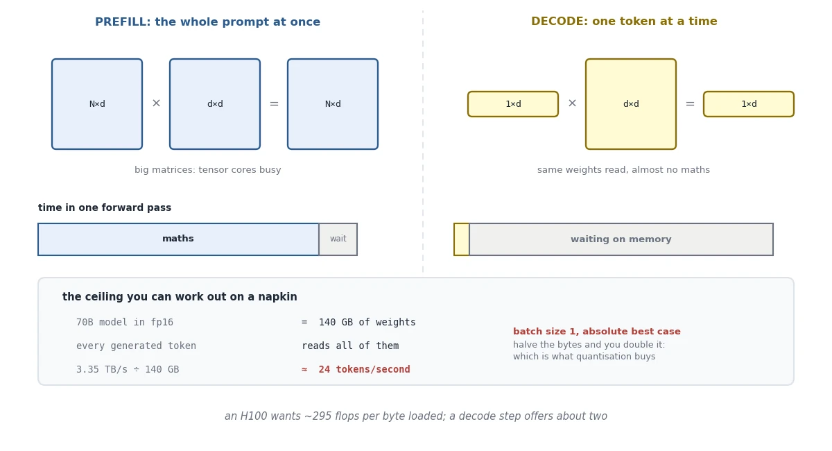
Same weights, same kernels, same GPU. Completely different bottleneck.

Work the numbers. Two figures from NVIDIA’s H100 SXM datasheet decide everything that follows (SXM is the version that plugs into a socket on the server board, as opposed to the PCIe card):

Figure	What it measures	Where it comes from
990 TFLOP/s	How much arithmetic the tensor cores can do: 990 trillion bf16 floating-point operations per second	The datasheet’s headline is 1,979, but that assumes 2:4 sparsity, which only applies to specially pruned weights that ordinary models do not have. Dense is half of it.
3.35 TB/s	How fast data moves from HBM (the GPU’s 80 GB main memory) to the chip: 3.35 trillion bytes per second	HBM3 memory bandwidth

bf16 is one of the reduced-precision float formats this series keeps returning to: bf16 (bfloat16, the 16-bit “brain floating point” format), fp16 (16-bit floating point) and fp8 (8-bit floating point). Part 5 gets into what those bits actually mean.

Divide one by the other:

  990 × 10¹² flop/s
 ───────────────────  =  295 flop/byte      (the "/s" cancels)
 3.35 × 10¹² byte/s

In the time HBM delivers one byte, the tensor cores could do about 295 operations. So a kernel has to do at least 295 flops of arithmetic per byte loaded to keep the tensor cores busy. Anything less, and the GPU spends time waiting on memory. This ratio is called the machine balance, and it is the corner of the roofline plot in Part 4.

A prefill GEMM (general matrix multiply, the operation tensor cores exist for) with a thousand rows clears that easily: each weight it loads is reused for all thousand tokens. A decode step is a matrix-vector product. Each fp16 weight (2 bytes) does one multiply and one add (2 flops), and then it is done:

batch 1:          2 flops ÷ 2 bytes  =   1 flop/byte  →  ~295× short
batch 64:    64 × 2 flops ÷ 2 bytes  =  64 flop/byte  →  ~5× short
batch 295:  295 × 2 flops ÷ 2 bytes  = 295 flop/byte  →  fully busy

(same bytes read every time; only the work per byte grows)

At batch size 1 you are roughly 300× short of what the machine wants. Arithmetic intensity grows one-for-one with the batch, which is why Part 4’s roofline puts “batch 1” at 1 flop per byte and labels its x-axis flops per byte = batch size.

The consequence is a hard ceiling you can compute on a napkin:

70B model in fp16  =  140 GB of weights
Every decode step reads ALL of them.

  3.35 TB/s ÷ 140 GB  ≈  24 decode steps/second
                          ^^^^^^^^^^^^^^^^^^^^^^
                          a ceiling: assumes full bandwidth,
                          ignores KV (key-value) cache reads and overhead

Batch size 1 is the worst case for the GPU, not the best. The ceiling above is about one user’s speed: every decode step streams all 140 GB, so no single conversation gets past ~24 tokens/s, whatever the batch. The GPU is a different story. At batch 1 it does one flop per byte, 295× less than it could, so every sequence you add rides along on the same weight read, until batch ~295, where compute catches up with memory.

Batch	Step time	Each user sees	GPU total	GPU busy
1	~42 ms	~24 tokens/s	~24 tokens/s	~0.3%
64	~42 ms	~24 tokens/s	~1,500 tokens/s	~22%
295	~42 ms	~24 tokens/s	~7,000 tokens/s	~100%

The weights never leave the GPU: they sit in HBM the whole time. The cost is moving them from HBM to the SMs, where the arithmetic happens. The chip’s on-chip memory (L2, shared memory and registers) totals about 115 MB, less than 0.1% of the model, and every one of those weights is used exactly once per token. By the time a weight is needed again, 140 GB has streamed past it, so no cache can help.

One simplification: 140 GB does not fit on a single 80 GB H100, so in practice the model is split across two or more GPUs, each reading its own share of the weights in parallel. Read the 24 as decode steps per second per 3.35 TB/s of bandwidth. Two H100s raise the ceiling to roughly 48, less the time spent communicating between them.

Two consequences fall straight out, and they are the economics of the entire industry:

Quantization helps decode enormously, and not for the reason people usually give. Going to fp8 halves the bytes and doubles the ceiling. It is not about compute; it is about bytes.

Batching is nearly free. Run 64 sequences together and you read those 140 GB once to produce 64 tokens instead of one. The memory clock does not move; only the arithmetic does, and you had arithmetic to spare.

This is why per-token pricing works at all. The marginal cost of the 64th concurrent user is close to zero, because they are riding along on a weight read you were already paying for. It is also why a single-user local deployment feels so much slower than a provider’s API (application programming interface) for the same model on the same hardware: you are paying the full memory bill for one token.

The KV cache

Without a cache, generating token t means recomputing attention over all t-1 previous tokens. With one (the KV cache, meaning the key and value projections each layer produces) you keep those projections and only compute the new token’s row.

bytes = 2 × layers × kv_heads × head_dim × dtype_bytes × seq_len × batch
        │     │         │          │           │           │        │
        │     │         │          │           │           │        └ number of sequences
        │     │         │          │           │           └ tokens in each sequence
        │     │         │          │           └ bytes per number (fp16 = 2)
        │     │         │          └ length of one key or value vector
        │     │         └ key/value heads per layer
        │     └ every layer has its own attention, so its own cache
        └ one key tensor + one value tensor (K and V)

The leading 2 is K and V: each layer stores a key and a value for every token. Queries are not cached, because a token’s query is used once, when that token is generated, while its key and value are read again by every token that follows.

For Llama-3-70B (80 layers, 8 KV heads via GQA, head dim 128, fp16) that is 2 × 80 × 8 × 128 × 2 bytes = 327,680 bytes, or 320 KB per token. The two 2s are unrelated: the first counts tensors (K and V), the second bytes per fp16 number. Switch to an fp8 cache and only the second one changes. GQA means grouped-query attention: it shares key/value heads across groups of query heads. An 8k conversation is 2.5 GB. A 128k one is 40 GB, on GPUs that already hold 140 GB of weights across a tensor-parallel group.

With plain multi-head attention instead of GQA, the same model would need 2.5 MB per token, eight times worse. Grouped-query attention, multi-head latent attention and fp8 KV caches are not micro-optimizations. They exist because this single term decides how many users fit on a GPU.

What an inference engine adds over model.generate()

model.generate(), the generation method in Hugging Face Transformers, runs the decode loop for one request in Python. An inference engine such as vLLM, SGLang (Structured Generation Language) or TensorRT-LLM runs it for every request on its GPUs at once, re-planning batch membership every single iteration. That re-planning is the whole product.

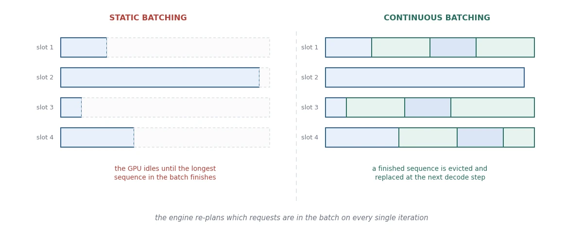Static batching cannot retire the batch until the longest sequence finishes.

The rest of the list all follows from prefill and decode being different:

• Speculative decoding. Decode leaves most of the GPU’s compute idle, so let a small draft model guess the next few tokens and have the big model check them all in one pass. Checking five tokens costs about the same as generating one, because the weight read is the same.
• Prefix caching. Requests that start with the same system prompt or chat history can share its KV cache and skip that prefill entirely. For chat and agent workloads this is often the biggest single win.
• Chunked prefill. One long prompt’s prefill would freeze every other user’s decode while it runs. Engines cut it into chunks and interleave them with decode steps.
• Prefill-decode disaggregation. The two phases want opposite hardware, so large deployments run them on separate pools of GPUs.

The engines

Engine	Signature idea	Where it fits
vLLM	PagedAttention, continuous batching	the general-purpose default; broadest model coverage
SGLang	RadixAttention prefix tree, fast constrained decoding	prefix-heavy, multi-turn, agentic, structured output
TensorRT-LLM	ahead-of-time compilation into a fused engine plan	standardized NVIDIA fleets, peak performance for a build step
llama.cpp / Ollama	GGUF (llama.cpp’s model file format), CPU and consumer GPU	local, single-user; not a fleet server
NVIDIA Dynamo	multi-node orchestration, KV-aware routing	the layer above the engines, at cluster scale

If you run this on Kubernetes

An inference server breaks most Kubernetes defaults, because those defaults assume an ordinary web service: starts in seconds, uses more memory and CPU under load, and every replica is interchangeable. None of that holds here.

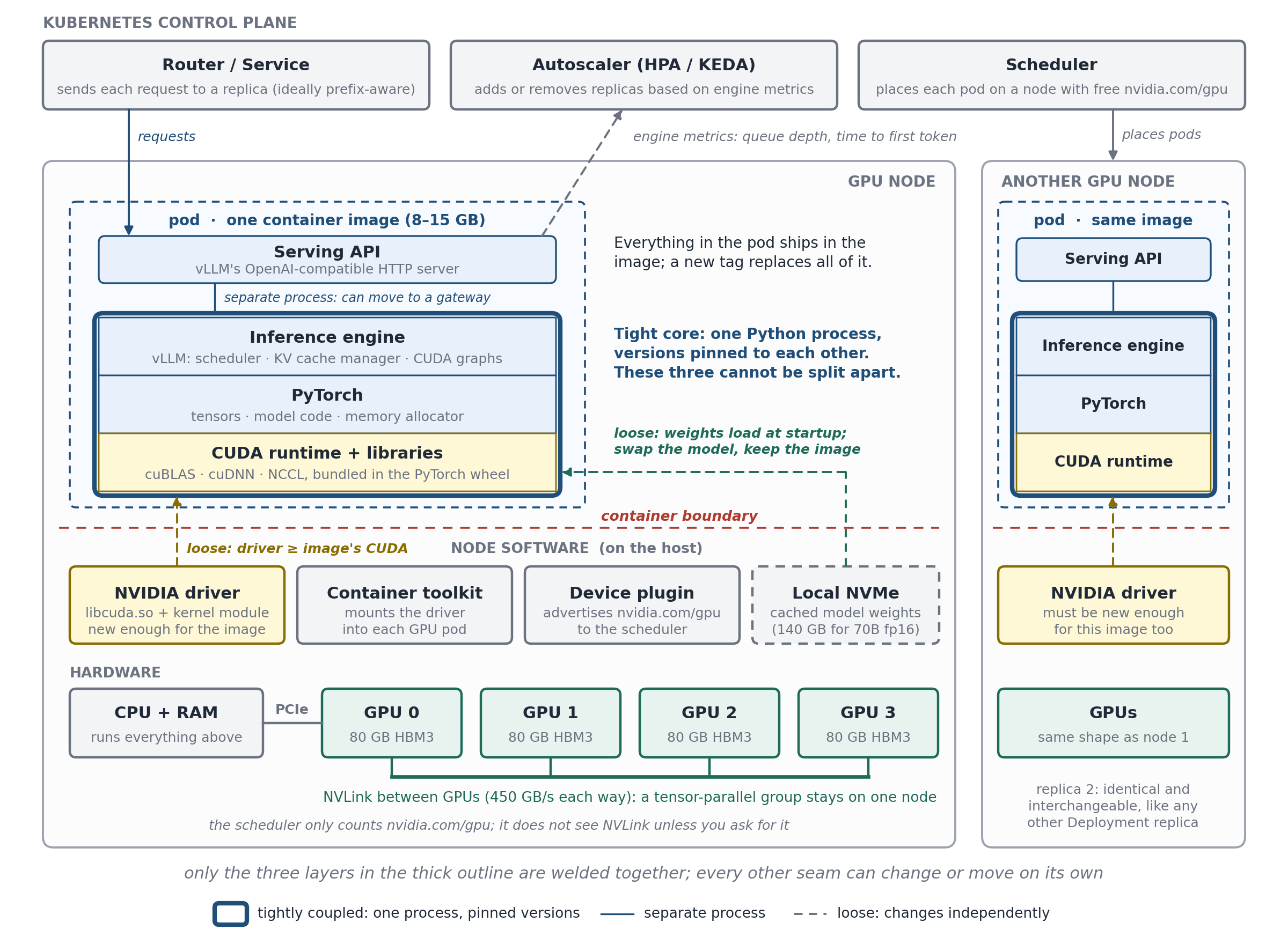The container image carries the top four layers, but only three of them are welded together: the engine, PyTorch and the CUDA runtime run in one process with pinned versions. The serving API, the driver and the weights are looser seams, and Kubernetes’ control plane decides where pods run and where requests go.

Starting a pod takes minutes, not seconds. The container starts quickly. Loading the weights doesn’t: a 70B model is 140 GB that has to be read from storage and copied into GPU memory, which takes anywhere from tens of seconds to several minutes, depending on where the weights live. Pre-pull the container image, keep the weights on the node’s local NVMe (Non-Volatile Memory Express) drive, a fast local SSD, rather than fetching them over the network, and be careful with scale-to-zero: whoever sends the first request after a quiet period waits for the whole load.

The two graphs you would normally autoscale on are both misleading.

GPU memory used is flat. At startup, vLLM reserves about 90% of GPU memory (the gpu_memory_utilization setting) and carves it into KV cache blocks it hands out itself. The graph shows 90% with zero users and 90% with five hundred.

GPU utilization is always high. The number nvidia-smi (NVIDIA’s command-line GPU status tool) reports is the share of time any kernel was running, not how much of the GPU was doing useful work. It samples the GPU many times a second and asks one yes/no question: was at least one kernel running? It never asks how many of the 132 SMs were in use, or whether they were computing or just waiting for data. A decode kernel stalled on HBM is still a running kernel, so every sample says yes. The batch 1 row of the table earlier makes this concrete: the dashboard says 100% while the tensor cores are about 0.3% busy.

For a truer picture, NVIDIA’s DCGM (Data Center GPU Manager) exporter reports SM activity, tensor-core activity and memory-bandwidth activity as separate metrics. During decode, memory bandwidth reads high and tensor-core activity sits near zero, which is the real story.

Scale on what users actually wait for. The engines publish Prometheus metrics that do track load:

Metric	What it tells you
Waiting requests (queue depth)	requests that could not join the batch yet; above zero for long means you need more replicas
KV cache usage	how full the cache pool is; near 100%, new requests start queueing
Time to first token	what users feel; it climbs as the queue grows

Feed these to the Horizontal Pod Autoscaler (HPA, through the Prometheus Adapter) or to KEDA (Kubernetes Event-Driven Autoscaling) instead of CPU or GPU metrics.

Keep split models on well-connected GPUs. A model split across GPUs with tensor parallelism exchanges results after every layer, so the link between those GPUs sits on the critical path of every token. NVLink moves 450 GB/s each way; PCIe manages about 64, roughly 7× less (see the memory hierarchy table). Kubernetes only counts GPUs, so request nodes whose GPUs are NVLink-connected. And if a model is too big for one node, its pods must be started together or not at all (gang scheduling, via tools like Kueue, Volcano or LeaderWorkerSet). Otherwise half the pods start, sit on their GPUs, and wait for the other half.

Don’t send traffic until the model is loaded, and don’t kill the pod while it is loading. A readiness probe that only checks “is the port open” can pass before the weights are loaded and the CUDA graphs captured, so requests arrive and hang for a minute or more. Point it at the engine’s health endpoint, which only succeeds once the model is ready. Give it a generous startupProbe too: otherwise the liveness probe decides the loading pod is dead, restarts it, and it never finishes loading.

Route follow-up requests back to the same replica. The second turn of a conversation contains the whole first turn as its prompt. The replica that served turn one still has that prefix in its KV cache (prefix caching, above), so it can skip most of the prefill. Round-robin load balancing sends turn two somewhere else, which recomputes everything from scratch. Route by conversation or by prompt prefix instead; this is what KV-aware routers such as NVIDIA Dynamo do.

Why does each layer depend on the next?

This was the question that unlocked the most for me. Why does vLLM need PyTorch? Why does PyTorch need CUDA? Why does CUDA need kernels?

The answer is that these are not the same kind of dependency, and the last one is not a dependency at all.

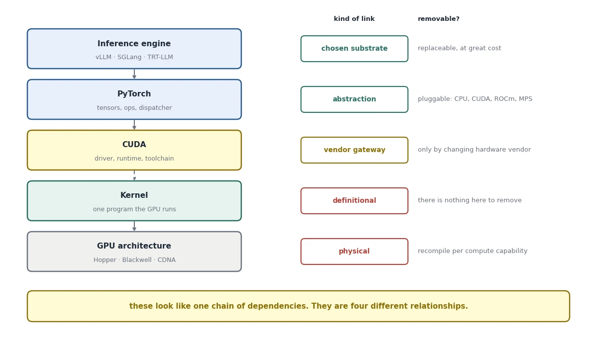Reading this as one chain is what made it confusing.

Engine → PyTorch: a build-versus-buy decision

The proof that this is a choice is that llama.cpp exists and has no PyTorch anywhere in it: it has its own tensor library, ggml, written from scratch in C. MLC-LLM (Machine Learning Compilation for LLMs) uses Apache TVM, a deep-learning compiler, instead.

If vLLM dropped PyTorch, it would have to rebuild five things it currently gets for free. Roughly from most work to least:

What PyTorch provides	In plain terms
Model code	Ready-made implementations of Llama, Qwen, Mixtral, DeepSeek, Gemma and a hundred other models, plus the code that loads their weight files and splits them across GPUs. This is the biggest reason engines stay on PyTorch.
Memory allocator	Asking CUDA for fresh memory is slow and can make the GPU pause. PyTorch keeps freed memory in a pool and hands it straight back out, so allocating is almost free. Every serving system needs this.
GPU-to-GPU communication	A model split across GPUs has to combine partial results twice per layer. PyTorch wraps NVIDIA’s library for this, NCCL (NVIDIA Collective Communications Library).
Other hardware	The same model code runs on AMD GPUs (through ROCm, AMD’s counterpart to CUDA), Google Tensor Processing Units (TPUs), Intel Gaudi and Huawei Ascend, without a separate version for each.
Tensors	The basic “array of numbers on the GPU” type: its shape, number format, and slicing without copying. Easy to write, but a lot of code for no competitive advantage.

None of that is what makes vLLM fast, though. PyTorch knows how to run one forward pass of one model on whatever batch it is handed. It has no idea that hundreds of users are waiting, that each conversation grows one token at a time, or that GPU memory has to be shared between them. Handling that is the engine’s job, and it is code vLLM writes itself:

What the engine builds	Why PyTorch can’t provide it
Scheduler	Decides every step which requests join the batch, which leave and which wait (continuous batching, above). PyTorch only sees the batch it is given.
KV cache manager	Reserves one large block of GPU memory at startup and hands it out in small pages as each conversation grows, instead of reserving room for the longest possible conversation up front. PyTorch’s allocator knows nothing about conversations.
Attention kernels	Hand-written kernels that read keys and values scattered across those pages. PyTorch’s built-in attention expects them in one contiguous array.
CUDA graph capture	Records each decode step once and replays it with a single launch (see How capture works above).
Serving features	Prefix caching, speculative decoding, chunked prefill, sampling, and streaming responses over an OpenAI-compatible API.

A rough split: PyTorch answers “how do I run this model once?”; the engine answers “how do I run it for everyone, continuously, without wasting memory or GPU time?”

But here is the structural detail I had missed: engines deliberately bypass PyTorch exactly where it would cost them.

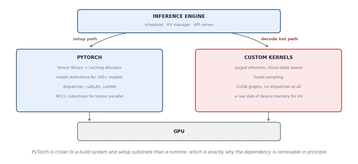The KV cache is not a PyTorch allocation, and once CUDA graphs are captured the decode step never touches the dispatcher.

The KV cache manager, the attention kernels and the CUDA graphs in that table are exactly the pieces that bypass PyTorch. PyTorch is closer to a build system and setup substrate for these engines than a runtime. That is exactly why the dependency is removable in principle, and why nobody bothers.

PyTorch → CUDA: a gateway, not a preference

Two separate reasons, worth keeping apart.

First, PyTorch does not depend on CUDA in general. It depends on having some device backend, and the dispatcher is the mechanism: it reads the device and dtype (data type) off the tensors and routes torch.matmul to the vendor’s own matrix-math library: cuBLAS on NVIDIA GPUs, hipBLAS on AMD GPUs, oneDNN (oneAPI Deep Neural Network Library) on CPUs, or MPSGraph (Metal Performance Shaders Graph) on Apple silicon. BLAS, in the first two, stands for Basic Linear Algebra Subprograms, the standard set of matrix and vector operations. PyTorch depends on a driver the way an application depends on a database driver: your app does not care whether it is Postgres or MySQL, but it needs one, and it has to match the database you actually have.

Second, once you have NVIDIA hardware, CUDA is the only door. A GPU is a separate device plugged into the PCIe slot, with its own memory that the CPU cannot read or write directly. To make it do anything, something has to reserve GPU memory, copy the data across PCIe into it, write the work out in the GPU’s own command format, put it in the GPU’s queue, and wait for the GPU to signal that it is done. That command format is proprietary, undocumented, and changes every architecture. The only supported entry point is libcuda.so, which ships with the driver.

CUDA → kernels: this one is a category error

CUDA does not depend on kernels the way vLLM depends on PyTorch. A kernel is the unit of work in the CUDA programming model.

The comparison that makes it click: a Pod is to Kubernetes what a kernel is to CUDA. You would not say Kubernetes depends on Pods. A Pod is the thing Kubernetes schedules.

The reason is architectural. A GPU is not a coprocessor you call functions on; it is a device you submit programs to. Its whole API surface reduces to about three verbs: allocate and free device memory, copy bytes across the bus, and launch a kernel. Every computation the GPU performs is a kernel launch, because the hardware has no other mechanism. It has 132 SMs that each need thousands of independent threads resident to hide memory latency, so work handed to it must arrive already shaped as a grid of independent blocks.

Why the chain feels so rigid in practice

PyTorch wheels (Python’s package format) bundle the CUDA runtime, cuBLAS, cuDNN (CUDA Deep Neural Network library) and NCCL; that is most of why a serving image is 8-15 GB. What you cannot bundle is the driver: libcuda.so lives on the host and gets injected by the NVIDIA container toolkit. Hence the classic failure where the image is fine but the node’s driver is too old.

Two version numbers that routinely confuse people. They come from the two halves of the CUDA layer in the stack diagram. nvidia-smi is NVIDIA’s command-line status tool; it is installed with the driver on the host and talks to the driver directly, so the “CUDA Version” in its header is the highest CUDA version that driver supports. torch.version.cuda comes from the CUDA runtime bundled inside PyTorch, in your image: it is the version PyTorch was built against.

Number	Comes from	Means
nvidia-smi	the driver, on the host	the newest CUDA this machine can run (its “CUDA Version” line)
torch.version.cuda	the CUDA runtime inside PyTorch, in the image	the CUDA this PyTorch needs

They differ all the time, and that is fine: the driver’s number must simply be ≥ PyTorch’s.

The tighter constraint is that vLLM and SGLang ship their custom kernels already compiled, and compiled code only works with the exact PyTorch and CUDA versions it was built against (technically, PyTorch’s C++ ABI, its application binary interface). So each piece pins the next, all the way down:

vLLM version     its compiled kernels work with one PyTorch version
     ↓
torch version    each PyTorch release is built for specific CUDA versions
     ↓
CUDA build       each CUDA version needs a minimum driver version
     ↓
driver           installed on the node, not in your image
     ↓
host image       a new driver usually means a new node image and a reboot

The top three travel together inside your container image. The driver belongs to the node. So upgrading an inference deployment is a coordinated change to four things (vLLM, PyTorch, CUDA and the node’s driver) rather than a version bump.

This is also how “just bump the image tag” breaks a cluster on a Friday. The new tag quietly upgrades vLLM, PyTorch and CUDA in one go. If that CUDA needs a newer driver than the nodes have, every new pod fails at startup with a CUDA error along the lines of driver version is insufficient, one replica at a time as the rollout proceeds. The safe order is bottom-up: upgrade the nodes’ driver first (a newer driver still runs older CUDA versions), then roll out the new image.

One exception worth knowing. Since CUDA 11, NVIDIA supports minor version compatibility: code built with a newer CUDA can often run on a slightly older driver, as long as both belong to the same major version (both 12.x, for example). So in practice the break usually comes when an image crosses a major CUDA version (11 to 12), or when its kernels rely on features only a newer driver provides. Check the minimum driver version in NVIDIA’s CUDA release notes rather than assuming either way.

What this sets up

Everything in this post reduced to the same sentence twice: decode reads all the weights to produce one token, and that read is the bill. Continuous batching, quantization, speculative decoding, prefix caching, GQA. Every one of them is an attempt to get more output per byte moved.

Part 3 goes one level down into the architecture itself, and answers a question that had been quietly bothering me: if decoder-only models threw away the encoder, where does the model’s understanding of your prompt actually live? The answer turns out to be the largest object in your GPU’s memory.

References

The book this series grew out of

1. Philip Kiely, Inference Engineering: Baseten Books, 2026.

GPU hardware and CUDA

2. NVIDIA, NVIDIA Hopper Architecture In-Depth: 132 SMs, 256 KB of L1/shared memory per SM, the 50 MB L2 cache and the register file.
3. NVIDIA, H100 Tensor Core GPU product page: the 3.35 TB/s bandwidth and the 1,979 TFLOP/s bf16 figure, which the spec table marks as “with sparsity”.
4. NVIDIA, Hopper Tuning Guide: up to 228 KB of shared memory per SM.
5. NVIDIA, CUDA Programming Guide: kernels, the execution model and the memory hierarchy.
6. Alan Gray, Getting Started with CUDA Graphs: launch overhead and how capture and replay remove it.
7. NVIDIA, CUDA Compatibility: how driver and CUDA versions must line up, including minor version compatibility.

Serving techniques

8. Efficient Memory Management for Large Language Model Serving with PagedAttention (Kwon et al.): the vLLM paper.
9. Orca: A Distributed Serving System for Transformer-Based Generative Models (Yu et al.): where continuous batching was introduced.
10. SARATHI (Agrawal et al.): chunked prefill.
11. GQA: Training Generalized Multi-Query Transformer Models from Multi-Head Checkpoints (Ainslie et al.): grouped-query attention.
12. Fast Inference from Transformers via Speculative Decoding (Leviathan et al.): speculative decoding.
13. SGLang: Efficient Execution of Structured Language Model Programs (Zheng et al.): RadixAttention and prefix sharing.
14. DistServe (Zhong et al.): prefill-decode disaggregation.

Software layers

15. PyTorch, CUDA semantics: memory management: the caching allocator.

Running it on Kubernetes

16. NVIDIA, nvidia-smi documentation: defines GPU utilization as the share of time one or more kernels was running.
17. NVIDIA, DCGM feature overview: the SM activity, tensor activity and memory bandwidth metrics.
18. vLLM, Metrics: the Prometheus metrics the engine exposes, including KV cache usage and time to first token.
19. NVIDIA, Container Toolkit and Kubernetes device plugin: how the driver reaches the pod and how GPUs reach the scheduler.
20. LeaderWorkerSet and KEDA: multi-node pod groups and event-driven autoscaling.

• llm
• inference
• vllm
• cuda
• gpu
• kv-cache
• kubernetes