Inference Engineering · Part 4 of 6

It's Memory Bandwidth All the Way Down

Tisan Das · Oct 1, 2026 · 20 min read

Contents

The idea here is simple, but memory bandwidth comes up so often in inference engineering that it deserves a post of its own. It rests on the split Part 2 drew between prefill and decode, and on the key-value (KV) cache Part 3 established as the largest object in GPU memory. If either is still fuzzy, read those first: everything here follows from them.

Two things had been nagging at me for a while. The first was the ops:byte ratio: floating-point operations (FLOPs) and bytes are not comparable, so dividing them looks like dividing apples and oranges. The second was the roofline plot, which also took some time to grasp.

Both cleared up the same way: we can stop staring at the ratio and the plot, and go back to milliseconds.

Disclaimer. This post is drafted with assistance from large language models (Claude Opus 5 and DeepSeek V4.1 Flash) based on conversations exploring LLM training and inference. All content has been reviewed, edited, and verified by a human author.

Is ops:byte even a valid ratio?

The objection is right on the surface, and wrong in practice, because nobody divides them and stops there. The ratio only ever appears on both sides of a comparison.

A GPU does two things at once: it computes, and it moves data. Those overlap, so runtime is whichever takes longer. A kernel has W flops to perform and Q bytes to move; the machine has peak compute F and peak bandwidth B.

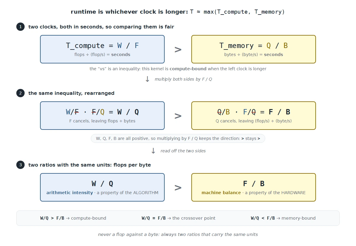The comparison is never a FLOP (one floating-point operation) against a byte. It is between two ratios that carry the same units.

The left side is flops divided by bytes. The right side is a rate divided by a rate: (FLOP/s) ÷ (byte/s). The seconds cancel, leaving flops per byte on both sides. For an H100 that machine number is 990 ÷ 3.35 ≈ 295 flops per byte.

What 295 means physically

By the time one byte travels from HBM (the GPU’s high-bandwidth main memory) to the chip, the tensor cores could complete about 295 flops. If an algorithm performs 1 flop per byte, 294 of those opportunities are wasted.

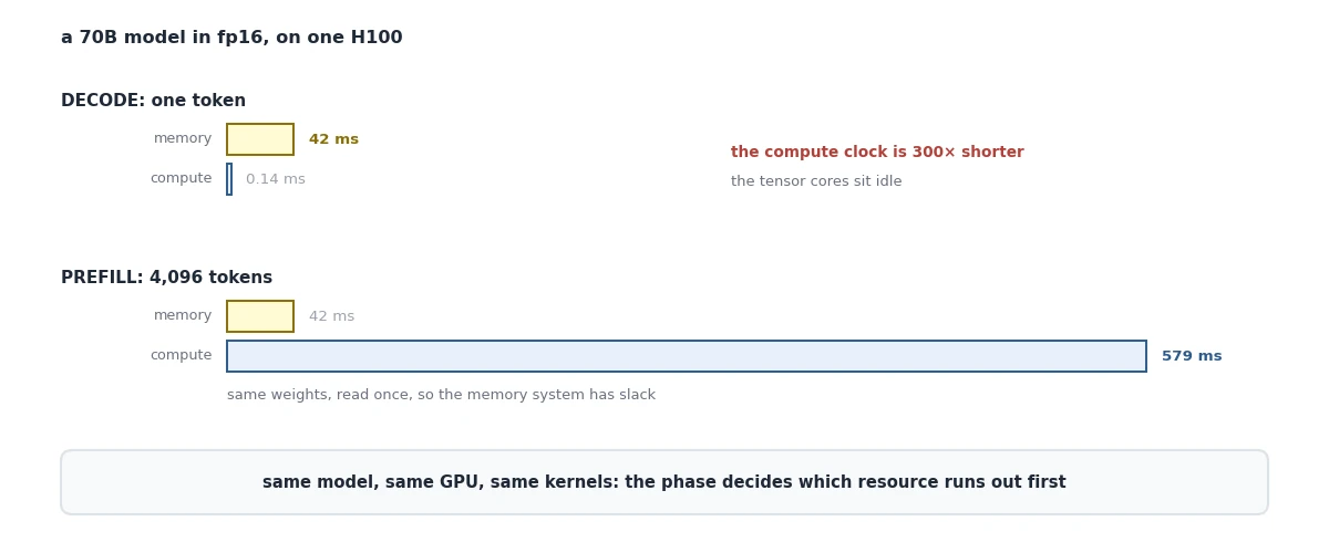Same model, same GPU, same kernels. The phase decides which resource runs out first.

Why a ratio rather than just measuring time? Because arithmetic intensity is a property of the algorithm alone, computable on paper before writing a line of code. Machine balance is a property of the hardware alone, available from a spec sheet. Comparing them predicts the bottleneck without running anything. More usefully, it tells which optimizations are pointless.

The balance point keeps moving

Device	Peak dense bf16	Bandwidth	Balance
V100	~125 TFLOP/s	0.9 TB/s	~139 flop/byte
A100 80GB	~312 TFLOP/s	2.0 TB/s	~153
H100 SXM	~990 TFLOP/s	3.35 TB/s	~295
H200 SXM	~990 TFLOP/s	4.8 TB/s	~206

From V100 to H100, compute grew roughly eightfold while bandwidth grew under fourfold. That is the memory wall: each generation demands more arithmetic intensity from the code just to stay busy.

H200 is the interesting row: the same compute as H100, but 43% more bandwidth. Inference, decode especially, is memory-bound: its arithmetic intensity sits far below the machine balance, so the tensor cores spend most of their time waiting on HBM. More compute would not help it; more bandwidth does. H200 is the chip built for exactly that.

The same comparison works at every link data crosses, not just HBM. Each link has its own bandwidth, so each has its own balance point: registers to SRAM (the on-chip scratchpad), SRAM to HBM, HBM to a peer GPU over NVLink, GPU to host over PCIe. The slower the link, the more work each byte crossing it has to pay for. Two familiar optimizations are this analysis applied at a specific link:

• Kernel fusion (SRAM/HBM). Unfused, each operation writes its result to HBM and the next one reads it straight back. Fusing them keeps the intermediate in SRAM, so the same flops cost fewer HBM bytes and intensity goes up.
• Tensor-parallel sizing (NVLink). Splitting a layer across more GPUs gives each one less compute, but they still exchange activations over NVLink at every layer. Past some point the exchange takes longer than the math, which is why tensor parallelism usually stops at one NVLink-connected node.

It is also structurally identical to a question any database person already asks: is this query CPU-bound or I/O-bound? The usual check is to compute cycles per byte read and compare it against the machine’s cycles per byte of I/O bandwidth. Nobody finds that comparison suspicious, and it is the same manoeuvre.

The roofline, derived from milliseconds

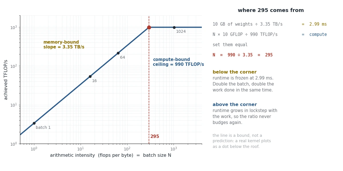
Take one H100, with 990 TFLOP/s of compute and 3.35 TB/s of HBM bandwidth, and a 5-billion-parameter model in fp16: 10 GB of weights. Run one decode step for a batch of sequences and time the two clocks.

The memory clock is fixed. The weights are read from HBM once per step and shared by every sequence in the batch, so the read costs 10 GB ÷ 3.35 TB/s = 2.99 ms whether the batch is 1 or 4,096.

The compute clock grows with the batch. Each weight does 2 flops (a multiply and an add) for every sequence, so a batch of N sequences needs 10 GFLOP × N.

One clock is fixed and the other keeps growing, so at some batch size they cross. Below that point the GPU is waiting on memory; above it, on compute. The table shows where.

Batch	Flops	Memory clock	Compute clock	Runtime	Work per second
1	10 G	2.99 ms	0.01 ms	2.99 ms	3.3 TFLOP/s
16	160 G	2.99 ms	0.16 ms	2.99 ms	54 TFLOP/s
64	640 G	2.99 ms	0.65 ms	2.99 ms	214 TFLOP/s
256	2.6 T	2.99 ms	2.59 ms	2.99 ms	858 TFLOP/s
295	3.0 T	2.99 ms	2.99 ms	2.99 ms	990 TFLOP/s
1024	10.2 T	2.99 ms	10.34 ms	10.34 ms	990 TFLOP/s
4096	41 T	2.99 ms	41.37 ms	41.37 ms	990 TFLOP/s

Read the last column down. Below 295 it doubles every time the batch doubles. Above 295 it stops moving.

Look at why, in the runtime column. Below 295, runtime is frozen at 2.99 ms: the GPU is waiting on HBM regardless, so doubling the batch doubles the work done in the same fixed time. Above 295, runtime grows in lockstep with the work, so the ratio never budges.

Plot that last column and the result is the roofline.

The roofline: bandwidth sets the sloped part, compute sets the flat roof, and they meet at 295 flops per byte.

Arithmetic intensity for this kernel is flops ÷ bytes = (10 GFLOP × N) ÷ 10 GB = N. The batch size is the arithmetic intensity. Change the x-axis label and the numbers do not move.

Why the plot is a min. Runtime is the max of the two clocks: the slower one sets the pace. The roofline plots throughput, which is work ÷ runtime, so the slower clock now gives the lower number. That makes throughput the min of two limits: what bandwidth allows (3.35 TB/s × intensity, the slope) and what compute allows (990 TFLOP/s, the flat roof). The line always follows whichever is lower. It’s the same table, read as time or as throughput.

How to actually use it

Count a kernel’s flops and bytes on paper, divide one by the other, and compare the result to the GPU’s balance point (295 on an H100). Then find the kernel on the plot: where it sits decides what helps. The line is a bound, not a prediction; a real kernel lands somewhere on or below it.

Counting by hand. For a matmul of an N × K input by a K × M weight: flops = 2 × N × K × M (one multiply and one add per weight, per row of input). Bytes = everything read plus everything written, 2 × (K·M + N·K + N·M) in bf16. For one 8192 × 8192 weight at batch 1, that is 134 M flops over ~134 MB: intensity ~1, deeply memory-bound. During prefill with 2,048 tokens, it is 275 G flops over ~201 MB: intensity ~1,370, compute-bound. Same matrix; only N changed.

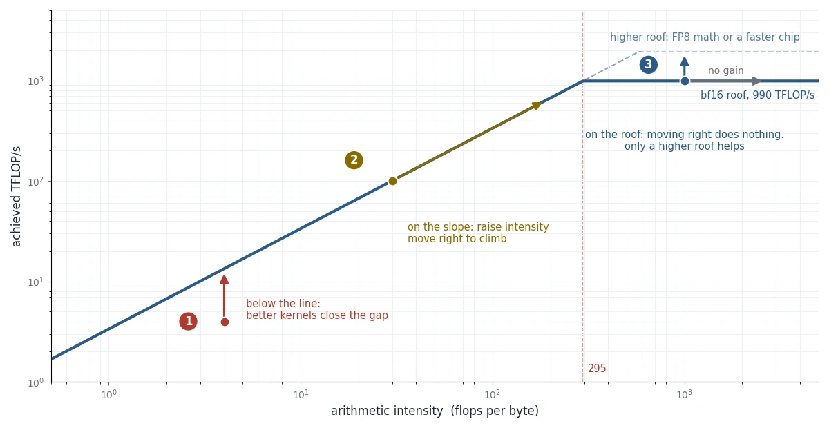Close the gap, move right, or raise the roof: which one helps depends on where the kernel sits.

1. Below the line: the gap is the implementation’s inefficiency. Better kernels close it.
2. On the slope: memory-bound. Raise intensity with bigger batches, lower-precision weights, or fused kernels. More tensor cores change nothing.
3. On the roof: compute-bound. Moving right gains nothing. Raise the roof with lower-precision math or a faster chip, or do fewer flops. More bandwidth changes nothing.

Smaller weights vs faster math. “Lower precision” means two different things in practice, and they fix different problems.

• Smaller weights (weight-only quantization, such as INT4 with AWQ or GPTQ). Each weight is stored in 4 bits instead of 16, so reading the weights from HBM moves a quarter of the bytes. Just before the multiply, the weights are converted back to bf16, so the math runs at the usual bf16 speed. Same work, fewer bytes: the dot moves right, and the roof stays where it was. This helps memory-bound kernels.
• Faster math (FP8). The weights and the activations they’re multiplied with are both in FP8, and the H100 has tensor cores that multiply FP8 numbers directly, about twice as fast as bf16. That raises the roof. FP8 weights are also half the size of bf16 ones, so the dot moves right too. This helps on both sides of the corner.

A quick way to tell them apart: what format does the multiply run in? If it’s still bf16, only the bytes got smaller.

FlashAttention vs PagedAttention

From the names, it’s easy to think of these two as competing approaches. However, they are not. They solve completely different problems at different layers, and every production stack uses both simultaneously.

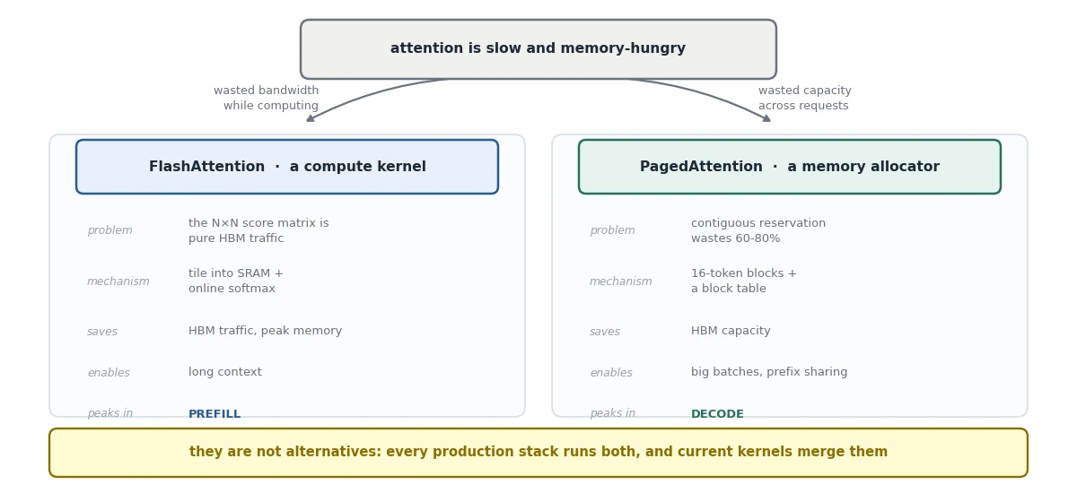In database terms: FlashAttention is getting a join to run inside the buffer pool instead of spilling to disk. PagedAttention is the buffer pool page manager itself.

FlashAttention’s problem

Attention is softmax(QKᵀ / √d) · V. To see why it is expensive, size every tensor for one attention head with two numbers: N = 4,096, the number of tokens in the sequence, and d = 128, the head dimension, meaning how many numbers each token’s query, key and value carry in one head (the same d as in √d). N sets the rows of every tensor; d sets the columns of Q, K and V. In fp16, each number takes 2 bytes:

Tensor	Shape (rows × columns)	Numbers	Bytes (× 2 in fp16)	Size
Q, K, V (each)	4,096 tokens × 128	524,288	1,048,576	~1 MB
Output O	4,096 tokens × 128	524,288	1,048,576	~1 MB
Scores QKᵀ	4,096 tokens × 4,096 tokens	16,777,216	33,554,432	33.5 MB

Q, K and V are small because each token contributes one row of 128 numbers. The model projects each token’s hidden state into a query, a key and a value, then splits each one across 32 heads of 128 numbers; a single head sees its 128. The score matrix is large because it has one entry for every pair of tokens: every query is scored against every key. Each of its rows holds 4,096 numbers instead of 128, which makes it 32 times the size of Q.

The same shapes, shrunk. Take 3 tokens and a head dimension of 4. For one head, Q is a table with one row per token:

	q₁	q₂	q₃	q₄
token 1	0.2	-1.1	0.7	0.0
token 2	0.5	0.3	-0.4	1.2
token 3	-0.9	0.8	0.1	0.6

That is 3 × 4 = 12 numbers, and K and V have the same shape. The score matrix is 3 × 3 = 9 numbers, one per query–key pair. At this size it is smaller than Q. At 4,096 tokens it is 32 times larger, because it grows with the square of the token count while Q grows linearly.

Written naively, attention runs as three separate kernels, and each one hands its result to the next through HBM:

Step	Reads from HBM	Writes to HBM
1. S = QKᵀ / √d	Q, K (2 MB)	S (33.5 MB)
2. P = softmax(S)	S (33.5 MB)	P (33.5 MB)
3. O = P · V	P (33.5 MB), V (1 MB)	O (1 MB)

The score matrix makes two round trips: written and read back for the softmax, then written and read back for the multiply by V. That is 4 × 33.5 MB ≈ 134 MB of traffic for matrices nobody wants to keep, against about 4 MB for Q, K, V and the output.

It is also quadratic. At N = 16,384 the score matrix is 16,384² × 2 bytes ≈ 537 MB per head per layer, or 17 GB per layer across 32 heads, before batching. That is why long context was out of reach before this.

Checking against the roofline: naive attention has an intensity of roughly d/2 = 64 flops per byte, well under 295. Squarely memory-bound, and the bytes are almost all wasted.

The obstacle is that attention cannot simply be tiled, because softmax normalizes over the entire row: the sum of exponentials across all N keys is needed before any single score can be normalized.

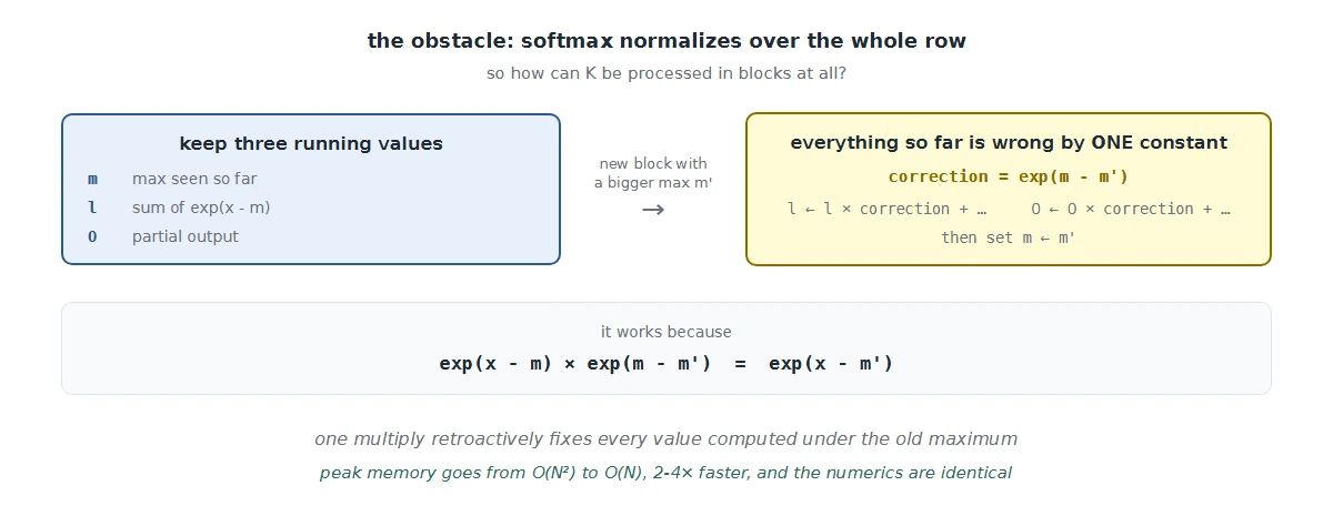Peak memory goes from O(N²) to O(N), typical shapes run 2-4× faster, and the numerics are identical.

That last property is why FlashAttention won so completely. It displaced an entire research family of sparse and linear attention approximations, because there is no accuracy trade-off to argue about: it computes exactly the same function, just without materializing the intermediate.

One more detail, this time from training. Training runs the model forwards and then backwards, and the backward step needs the attention scores again. There are two ways to have them ready:

• Store them. Write the 33.5 MB score matrix to HBM during the forward pass and read it back later: 33.5 MB written + 33.5 MB read = 67 MB of traffic, and 67 MB ÷ 3.35 TB/s ≈ 20 µs on an H100.
• Recompute them. Keep only Q and K, which are about 1 MB each and kept anyway, plus one small number per row from the softmax. Redo QKᵀ in SRAM when it’s needed: 2 × N × N × d = 2 × 4,096 × 4,096 × 128 ≈ 4.3 GFLOP, and 4.3 GFLOP ÷ 990 TFLOP/s ≈ 4.3 µs.

FlashAttention recomputes. Doing the same math twice sounds wasteful, but it is about five times faster than the round trip, because the GPU is far quicker at arithmetic than at moving bytes. That is the roofline again: when a kernel is memory-bound, spare compute is cheap and bytes are expensive.

PagedAttention’s problem

Completely different. Fifty concurrent users, each conversation growing unpredictably, each token costing ~320 KB of KV cache.

Where the 320 KB comes from. It is for Llama-3-70B, the model Part 2 worked it out for. For each token, the KV cache stores one key and one value per KV head, in every layer:

2 (K and V) × 80 layers × 8 KV heads × 128 numbers per head × 2 bytes (fp16) = 327,680 bytes ≈ 320 KB

• 2 (K and V): the cache holds two tensors, keys and values.
• 80 layers: every layer keeps its own keys and values.
• 8 KV heads: Llama-3-70B uses grouped-query attention (GQA), so its 64 query heads share only 8 key/value heads. Without GQA, the cache would be 8 times bigger, about 2.5 MB per token.
• 128: the head dimension, the same d = 128 as in the FlashAttention section.
• 2 bytes: each number takes 2 bytes in fp16.

327,680 bytes is exactly 320 KiB (327,680 ÷ 1,024), which is why the number comes out so round.

Per token that sounds small, but it adds up fast. An 8k-token conversation holds 2.5 GB of cache; fifty of them hold 125 GB. And none of those conversations knows in advance how long it will get, so the server cannot know how much memory each one needs.

The question PagedAttention answers is how to lay all of that out in memory. The obvious approach reserves one contiguous region per request, sized for the longest output it might produce, because the attention kernel wants K and V as regular strided tensors.

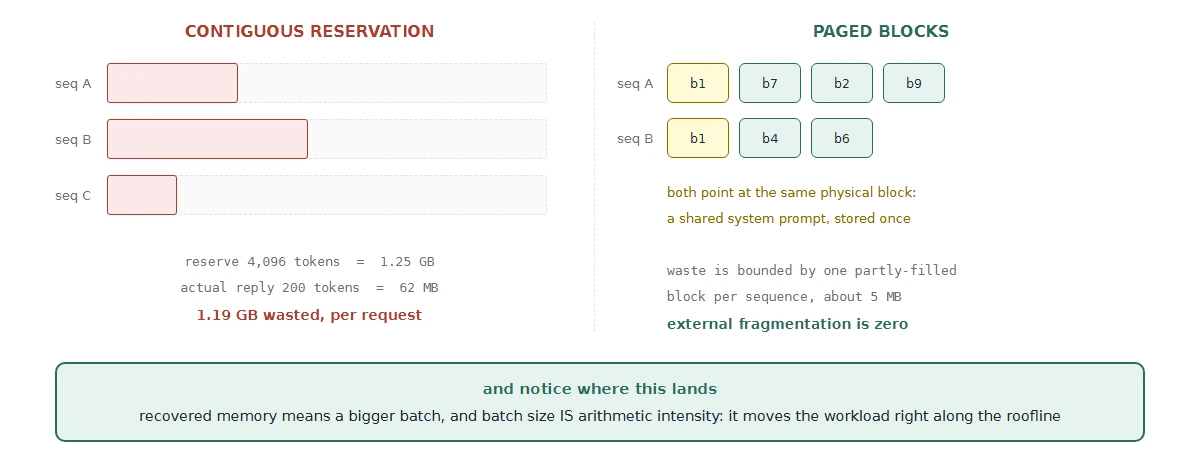The vLLM paper measured existing systems storing useful tokens in only 20.4-38.2% of allocated KV memory.

The fix is exactly OS virtual memory: cut the cache into fixed 16-token blocks, give each sequence a block table, allocate on demand, and let the kernel gather K and V through that table. Waste is now bounded by at most one partially-filled block per sequence, and external fragmentation is zero because every block is the same size.

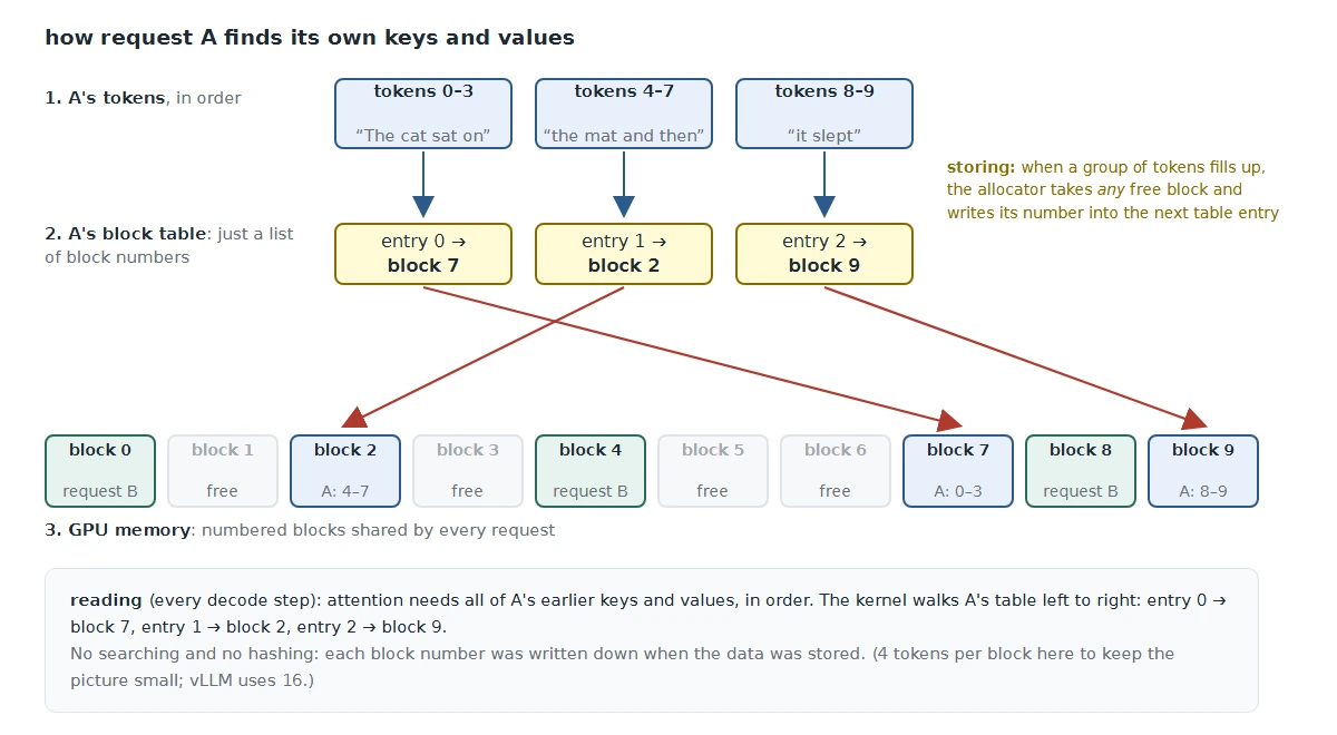A block table works like a coat-check ticket: the block number is written down when the data is stored, so finding it later is a plain array read, not a search.

The indirection buys sharing. Because a block table only points at physical blocks, two tables can point at the same block. A shared block is copied only when one of them needs to write into it (copy-on-write). Two features follow with almost no extra work:

• Prefix caching. Requests that start with the same system prompt share its blocks instead of each storing a copy.
• Parallel sampling. Asking for several different answers to one prompt (the n parameter in OpenAI-style APIs). Every answer shares the prompt’s blocks and allocates new ones only for its own tokens.

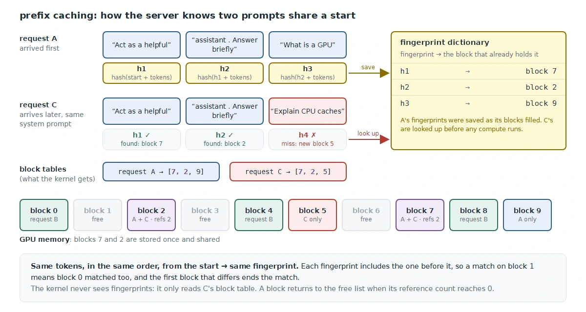How prefix caching finds the shared part: each full block gets a fingerprint chained to the one before it, so a match means the whole prompt up to that block is identical. The match happens once, when the request arrives; the kernel only ever sees block tables.

And notice where this lands. Recovered memory means a bigger batch, and batch size is arithmetic intensity in decode. PagedAttention’s real payoff is not saving memory for its own sake: it moves the workload further right along the roofline diagonal.

They peak in different phases

During prefill there are thousands of query tokens at once, so the score matrix really is N×N and FlashAttention’s tiling is the whole game. During decode there is a single query token, so the scores are just 1×N: there is no big matrix to avoid, and FlashAttention’s core benefit largely evaporates. What matters in decode is juggling dozens of independently growing caches, which is PagedAttention’s problem exactly.

Current kernels merge both ideas: FlashAttention-2/3, FlashInfer and vLLM’s own paged kernels all tile into SRAM and stream the softmax while fetching K and V through a block table. This combination is often called paged FlashAttention.

The only real friction is that every K and V read now goes through the block table first, an extra hop in reads that FlashAttention wants perfectly coalesced. That hop is a plain array read, like an OS page table. The fingerprint hashing from prefix caching does not happen here: it ran once, when the request arrived, and only decided which block numbers went into the table. Implementations absorb the hop by keeping blocks large enough that each still yields a clean contiguous burst.

What this sets up

The rest of the series uses the roofline without deriving it again.

Part 5 applies it somewhere unexpected: the sampling settings temperature, top_k and top_p. On their own they are simple arithmetic on a list of numbers and take microseconds. The catch is the size of that list. At every step, the model outputs one score (a logit) for every token in its vocabulary: about 128,000 numbers per sequence, or 512 KB in fp32.

Three things make that expensive:

• It grows with the batch. The weights are read once and shared by every sequence, but each sequence has its own logits. At batch 256, that is 128 MB.
• It lives in HBM. Every pass over the logits is a full read from memory.
• Sampling needs several passes. Scaling, filtering and picking a token each touch the list again.

So a question that sounds trivial, “how to find the largest k of 128,000 numbers”, becomes a real engineering problem. Answering it goes all the way down to how a floating-point number is laid out in memory.

References

1. Philip Kiely, Inference Engineering: Baseten Books, 2026.
2. Roofline: An Insightful Visual Performance Model (Williams, Waterman, Patterson): predates GPUs in this form and is still the clearest treatment.
3. FlashAttention (Dao et al.): tiling and online softmax, with the IO-complexity analysis.
4. Online normalizer calculation for softmax (Milakov & Gimelshein): the running-max trick on its own.
5. Efficient Memory Management for LLM Serving with PagedAttention (Kwon et al.): including the fragmentation measurements.

• llm
• inference
• roofline
• gpu
• flashattention
• pagedattention
• performance