Production RAG - Part 4: Hybrid Search, Fusion and Reranking

Ask a RAG system “how do I shut down an instance” and keyword search returns nothing useful, because the documentation says “halt” and “stop”. Ask it about CEAMVCSRE3110002C and semantic search drifts off into vaguely similar identifiers while keyword search finds the exact page instantly. Neither retriever is better. They have mirror-image blind spots, which is the entire argument for running both and merging the results.

Part of the Production RAG series (9 parts)

1. Production RAG - Part 1: Anatomy of the Pipeline
2. Production RAG - Part 2: Extracting Trustworthy Text from PDFs
3. Production RAG - Part 3: Chunking for Retrieval
4. Production RAG - Part 4: Hybrid Search, Fusion and Reranking ← you are here
5. Production RAG - Part 5: Images and Multimodal Retrieval
6. Production RAG - Part 6: Entities and Knowledge Graphs
7. Production RAG - Part 7: Grounded Generation
8. Production RAG - Part 8: Evaluation and Operations
9. Production RAG - Part 9: Splitting an Answer into Claims

Disclaimer. This post is drafted with assistance from large language models (Claude Opus 4.8 and DeepSeek V4 Pro) based on conversations exploring production RAG concepts. All content has been reviewed, edited, and verified by a human author.

Embeddings and the dot product

An embedding maps text to a dense vector so that semantic proximity becomes geometric proximity. Retrieval ranks by cosine similarity — the angle between two vectors, ignoring magnitude.

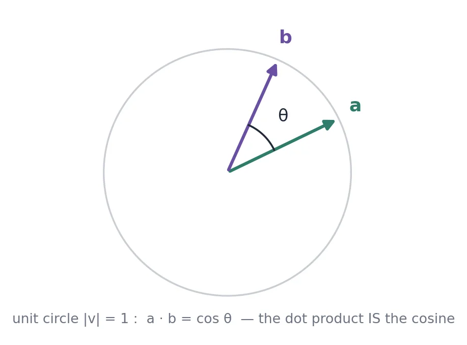
When vectors are normalized to unit length, the dot product is the cosine.

The identity a·b = |a||b|cos θ means that if both vectors have length 1, the dot product is the cosine. This is why production embedding models ship unit vectors: similarity becomes a bare dot product, which enables fast maximum-inner-product search, and magnitude noise disappears so only direction — meaning — matters.

A sentence-transformer bi-encoder works in four steps: tokenize the text, run the transformer, average the token vectors, normalize the result. The averaging step exists because a transformer emits one vector per token, not one per sentence — the mean is what collapses many vectors into one. Quality does not come from that averaging, though; it comes from contrastive fine-tuning, which trains the model on example pairs until paraphrases land close together and unrelated text lands far apart. all-MiniLM-L6-v2 emits 384 dimensions and accepts 256 tokens — anything longer is silently truncated, not chunked. Chunking is the ingestion layer’s job, and a model that drops the second half of your chunk will not tell you about it.

The well-known blind spot: negation. “Start the cluster” and “stop the cluster” embed close together, because they share almost everything except the one word that inverts the meaning.

The embedding model is coupled to the store. Queries must be embedded at search time by the same model and version that embedded the documents. Persist with one and reload with another and you get a silent failure — no error, just garbage similarity scores. Pin the embedding model version alongside the index, and store it on every row.

If you move embeddings between services, skip JSON: it inflates floats three to four times. Base64 of the raw bytes is a fixed 1.33x and bit-exact — but decoding requires agreeing on dtype, endianness and count. In Python that is np.frombuffer(b, '<f4'); in Go it is base64.StdEncoding plus binary.LittleEndian plus math.Float32frombits, never a float32() cast.

Sparse and dense

	Sparse (BM25)	Dense (embeddings)
Dimensionality	Vocabulary size, mostly zeros	384–4096, all non-zero
Matches on	Shared tokens	Meaning and proximity
Wins on	IDs, codes, proper nouns, rare exact strings	Synonyms, paraphrase
Blind to	Synonyms	Rare exact strings

What makes keyword search fast is the inverted index: a map from term to the list of documents containing it — the transpose of the sparse term-document matrix. You touch only the query’s terms, never the whole corpus. That is what powers FTS5 and every other BM25 engine.

Dense retrieval has no such shortcut, so exact nearest-neighbour search is O(N) per query. HNSW brings that to roughly O(log N) by combining a navigable small-world graph with a skip-list hierarchy of layers.

Parameter	Controls	Trade-off
M	Links per node	Higher = better recall, more memory
ef_construction	Build-time search width	Higher = better graph, slower build
ef_search	Query-time search width	Higher = better recall, slower query

sqlite-vec does brute-force KNN, which is entirely fine up to roughly 10⁵–10⁶ vectors. Past that, graduate to an HNSW index — pgvector, Qdrant, Weaviate — where the graph prunes the search instead of scanning every vector. Choosing the distributed vector database on day one is a common way to spend three weeks on a problem you do not have yet.

BM25 from scratch

The sparse arm needs a number per chunk per query term. BM25 produces that number, and understanding how — rather than treating it as a black box — explains why short chunks outscore long ones at the default settings, and why common English words can cost a chunk points.

Building the score in five steps

Query: cat. Index average length: 20 words. Four documents: A (1 word, 1 match), B (10 words, 1 match), C (20 words, 1 match), D (60 words, 3 matches).

1. Does the word appear? Score = 1 if present. A = B = C = D = 1. Four-way tie — too coarse.

2. Count the appearances. A = 1, B = 1, C = 1, D = 3. D wins. But paste B three times: 30 words, 3 matches, score 3 — tied with D despite no new information. Raw counting rewards length.

3. Divide by length. A: 1/1 = 1.0, B: 0.1, C: 0.05, D: 0.05. Overcorrected — A at density 1.0 is unbeatable, and D’s three matches vanished.

Two broken extremes: counting favours long documents, density favours short ones.

4. Blend the two. Divide by scale = (1 - b) + b × (length / avg_length). At b = 0, length is ignored. At b = 1, full density. Anything between is a partial correction. A document of exactly average length always gets scale = 1 regardless of b — the average is the pivot.

5. Cap the repeats. Put the count in numerator and denominator: tf × (k1 + 1) / (tf + k1 × scale). At k1 = 1.2 the ceiling is 2.2 — no chunk can ever score above 2.2 on a single query term.

The assembled formula

                N - n + 0.5           tf × (k1 + 1)
score = log( ----------------- ) × ---------------------------------
                  n + 0.5            tf + k1 × ((1-b) + b·|D|/avgdl)

the problem	the fix in the formula
Count the matches	tf on top
Stop paying for repeats	tf + k1 underneath — saturation
Adjust for length	(1-b) + b·len/avg — the dial
Weight by word rarity	The IDF multiplier out front

The standard settings are k1 = 1.2, b = 0.75. At average length the score is 1.00. Shorter documents score higher; longer ones lower. The crossover where a one-word document beats a genuinely relevant longer one has already happened at b = 0.75 — which is exactly the chunking problem part 3 describes.

IDF: weighting by word rarity

For a single-word query, IDF is a constant multiplying everything — it cannot reorder results. It only matters once the query has two or more words and you need to decide which match counts more.

If a word appears in n of N documents, classic IDF is log(N/n). BM25 uses an odds ratio instead: log((N - n + 0.5) / (n + 0.5)), descended from the Robertson–Sparck Jones relevance weight. The 0.5s are smoothing constants that keep the formula finite at the extremes.

IDF across a vocabulary

N = 1,000 documents:

term	n	IDF
the	990	−4.55
data	500	0.00
revenue	120	+1.99
mumbai	40	+3.17
polydactyl	2	+5.99

The zero crossing is exact: IDF = 0 when n = N/2. data at 500/1,000 landing on 0.00 is not rounding.

Negative IDF

Beyond n = N/2 the odds form goes negative — matching a query term costs points. In an index of English prose, the, of and is are in well over half your chunks. Classic log(N/n) merely decays to zero; the odds form makes common words actively harmful.

Implementations patch it:

• Lucene / Elasticsearch use log(1 + (N - n + 0.5)/(n + 0.5)), keeping the result always positive.
• FTS5 appears to clamp non-positive IDF to a small constant.
• Others floor at zero or clamp to an epsilon.

The tokenizer decides what IDF can ever see

All of that arithmetic runs on whatever the tokenizer handed over, and FTS5’s default unicode61 treats -, _ and . as separators. So us-east-1 never enters the index as a term at all — it enters as us, east and 1. Each of those is common enough in a cloud corpus to sit near or below the zero crossing, which means the most discriminative string in the query contributes almost nothing to the score, and can even cost points. The same happens to error_code and to every SKU, region code and resource id you have.

The repair is one tokenizer argument — tokenize = "porter unicode61 tokenchars '-_'" — which promotes - and _ from separators to word characters. us-east-1 becomes a single rare term with the high IDF it should have had all along. The trade is that east on its own no longer matches it, which is the right default for an identifier. The DDL below carries the change.

Do not add . to tokenchars. It looks like the obvious way to keep 17.20 in one piece, and it quietly wrecks ordinary prose: a sentence-ending period becomes part of the word before it, so a chunk ending “check the pool size first.” indexes the term first. and a user searching for first matches nothing at all. Nothing errors, and the loss is invisible because it only affects the last word of every sentence. Keep version strings findable by indexing their alternate forms instead — the alias expansion in part 6.

IDF does not rescue short chunks

IDF and length normalisation are separate multiplicative factors — neither undoes the other. For a single-term query IDF is constant and the 42-character fragment from part 3 still wins by nearly 2x. But term coverage partially does: BM25 sums per word, and a 42-character orphan row can only match one query term while the full table matches that term and others from its header. The orphan’s lead narrows from ~2x to roughly 1.4x — still losing, but an argument for keeping headers and captions inside the chunk.

Both arms in one SQLite file

CREATE TABLE chunks(id INTEGER PRIMARY KEY, doc_id TEXT, text TEXT);
CREATE VIRTUAL TABLE chunks_fts USING fts5(
  text, tokenize = "porter unicode61 tokenchars '-_'"
);
CREATE VIRTUAL TABLE chunks_vec USING vec0(embedding float[384] distance_metric=cosine);

-- BM25: scores are NEGATIVE in FTS5, more negative = better
SELECT rowid, bm25(chunks_fts) AS score FROM chunks_fts
WHERE chunks_fts MATCH ? ORDER BY score LIMIT ?;

-- Semantic: sqlite-vec KNN; smaller distance = closer
SELECT rowid, distance FROM chunks_vec
WHERE embedding MATCH ? AND k = ? ORDER BY distance;

The two virtual tables join on a shared rowid. Two operational details are easy to get wrong:

FTS5’s bm25() hardcodes k1 = 1.2 and b = 0.75. The function arguments are per-column weights, not model parameters. If you want to tune b — and for chunked corpora, b in the 0.3–0.4 range better reflects that chunk length is splitter noise rather than author signal — you need to leave FTS5 for Tantivy, Lucene, or a hand-rolled scorer. And FTS5 returns negated scores: more negative is better. Inverting the sign by accident produces a system that confidently retrieves the least relevant chunks, and everything downstream still works, so nothing errors. Worth a unit test on a known ranking.

Fusion: RRF

Fusion merges two ranked lists into one. It is important to be clear about what it does not do: it adds no new relevance signal, it only recombines rankings the retrievers already produced.

Reciprocal Rank Fusion:

score(d) = SUM over lists L of  1 / (k + rank_L(d))       # k ≈ 60

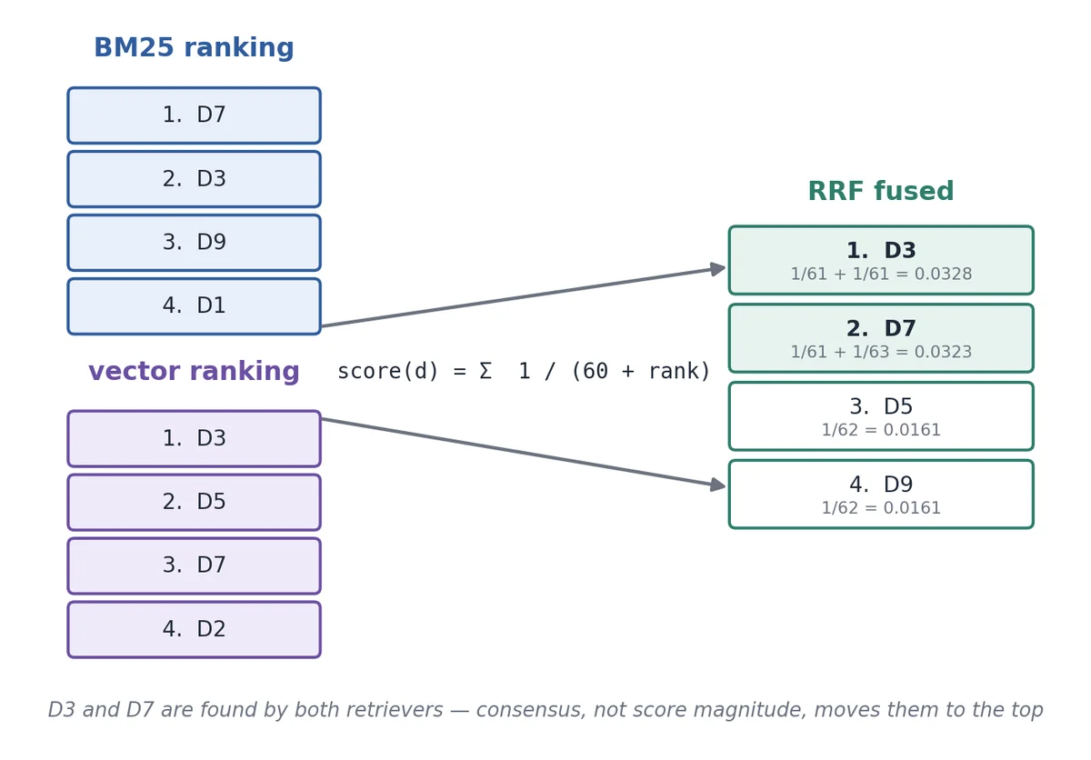RRF uses ranks only. Documents found by both retrievers rise, without any score normalization.

	RRF	Weighted average
Uses	Ranks	Raw scores
Needs normalization	No	Yes, and min-max is fragile
Document missing from one list	No penalty	Imputed as 0, so penalized

RRF rewards consensus and handles a single-list find gracefully — an additive bonus, never a penalty. It also avoids the entire question of how to compare a negative BM25 score with a cosine distance, which is a genuinely annoying problem to solve properly.

Fusion cannot fix a shared mistake. When both retrievers have the same blind spot — negation is the classic — both rank the wrong chunk highly, and RRF’s consensus reward amplifies the error. Fusion has no independent view of relevance. Only a reranker does. That is the core reason you still need one after RRF.

Fusion also cannot fix BM25’s length-normalisation inflation. A weighted average of raw scores lets the inflated 1.65 leak straight into the fused result. RRF is safer because it consumes ranks only — but the orphan is still rank 1 on the lexical side, so its rank contribution is undiminished. Fusion caps the damage; only the reranker repairs it.

Reranking

A reranker re-scores one candidate list using a stronger, independent judgment. Unlike fusion, it generates a genuinely new signal by re-reading the query against each document — and it uses the opposite architecture from the retriever.

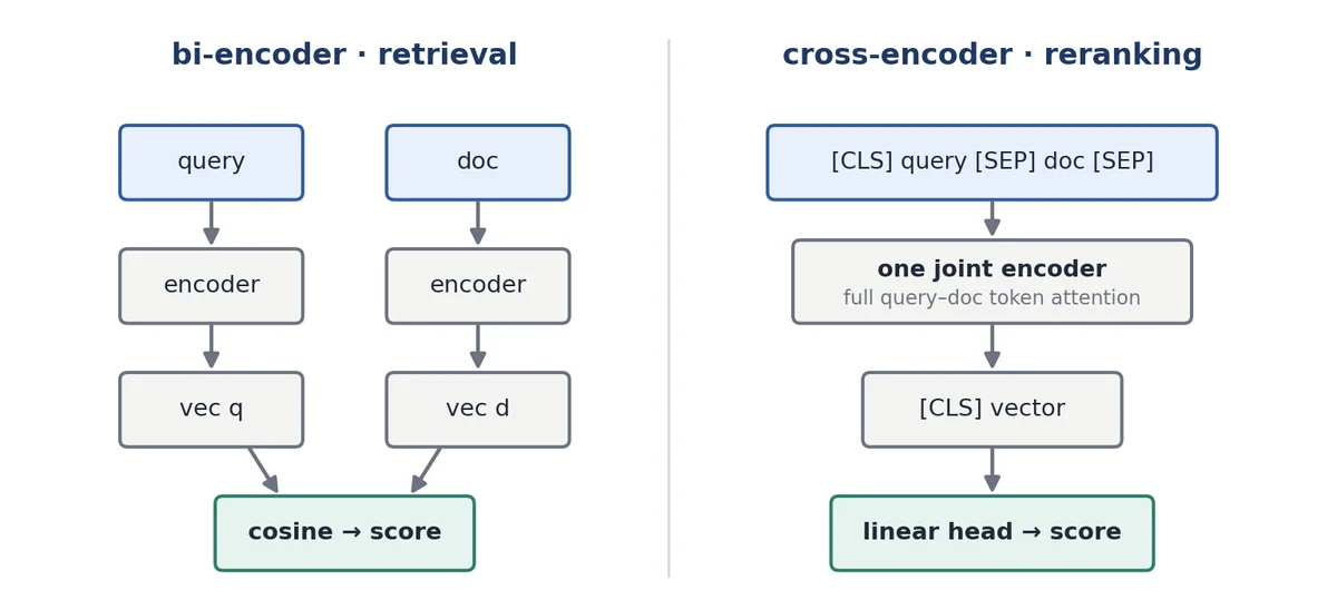Bi-encoder: encode separately, compare with cosine — scalable. Cross-encoder: encode jointly, read a score off [CLS] — accurate.

The cross-encoder concatenates [CLS] query [SEP] doc [SEP] into a single sequence, so every query token attends to every document token, and a linear head emits one relevance score. That token-level interaction catches exactly what a bi-encoder cannot: “stop” contradicting “start”, a qualifier that inverts a claim, a date that does not match.

The framing worth internalising is that embedding similarity is computed post hoc between two independently encoded texts, and never exploits the attention mechanism at all. Joint encoding does. The price is one forward pass per candidate, which is why a reranker runs on the top-N shortlist and never on the corpus.

MMR, the diversity reranker

Maximum marginal relevance dates to 1998 — redundancy in search results long predates LLMs. It reorders for coverage rather than relevance: each candidate earns points for query relevance and loses points for similarity to what has already been picked.

MMR(d) = λ · sim(d, q)  -  (1 - λ) · max sim(d, d_selected)

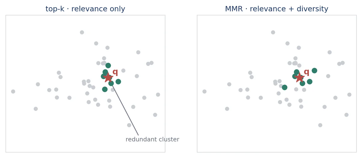Top-k clusters near-duplicates around the query; MMR spreads its selections across the candidate cloud.

This matters more than it looks. Five chunks saying the same thing waste your context budget and give the generator no new information, while a sixth chunk holding the qualifier that changes the answer sits just below the cutoff.

Chaining rerankers

Production stacks chain rerankers, because each one optimizes a different objective and the order is not commutative.

Stage	Optimizes	Scope	Pool
1. Cross-encoder	Relevance	Per-chunk	50 → 20
2. MMR	Diversity	Per-set	20 → 8
3. Custom rules	Business logic	Domain	8 → 5

Three principles fix that order. Run cheap-and-crude before expensive-and-precise, on progressively smaller sets. Run diversity on an already relevant set, or MMR will faithfully diversify garbage. And put hard business rules last — permission filtering especially — so that nothing downstream can override them.

Running a cross-encoder from Go

There is no first-class pure-Go cross-encoder: the tokenizer, the model and the forward pass are Python and PyTorch machinery. Three options:

Option	Shape	Verdict
ONNX export	onnxruntime bindings plus a Go tokenizer	Real, but CGo and tokenizer-drift risk
Python sidecar	Wrap in FastAPI, call over localhost	Recommended — zero drift
Hosted API	Managed rerank endpoints	Least code; data leaves the box

from fastapi import FastAPI
from sentence_transformers import CrossEncoder

model = CrossEncoder("cross-encoder/ms-marco-MiniLM-L-6-v2")
app = FastAPI()

@app.post("/rerank")
def rerank(body: dict):
    pairs = [(body["query"], c) for c in body["chunks"]]
    return {"scores": model.predict(pairs).tolist()}

The tokenizer-drift risk in the ONNX path is worth spelling out: if your Go tokenizer disagrees with the one the model was trained with — on a subword split, on Unicode normalization, on how it handles an unknown character — scores degrade quietly and only on the inputs where they disagree. The sidecar costs one hop and removes the entire class of problem.

What comes next

The next post leaves text behind and looks at images, tables screenshotted into PDFs, and why the architecture that is cheapest to ingest is usually the most expensive to run.

References

1. Ofer Mendelevitch and Forrest Sheng Bao, Hands-On RAG for Production, O’Reilly Media, 2026
2. Cormack, Clarke and Buettcher, Reciprocal Rank Fusion Outperforms Condorcet and Individual Rank Learning Methods, SIGIR 2009
3. Carbonell and Goldstein, The Use of MMR, Diversity-Based Reranking for Reordering Documents and Producing Summaries, SIGIR 1998
4. Malkov and Yashunin, Efficient and Robust Approximate Nearest Neighbor Search Using Hierarchical Navigable Small World Graphs, IEEE TPAMI 2020
5. Khattab and Zaharia, ColBERT: Efficient and Effective Passage Search via Contextualized Late Interaction over BERT, SIGIR 2020
6. Sentence-Transformers cross-encoder documentation
7. Robertson, S. E. and Sparck Jones, K. “Relevance weighting of search terms.” Journal of the American Society for Information Science, 1976
8. Robertson, S. and Zaragoza, H. “The Probabilistic Relevance Framework: BM25 and Beyond.” Foundations and Trends in Information Retrieval, 2009