Production RAG - Part 2: Extracting Trustworthy Text from PDFs

A PDF is not a document in any structured sense. Rooted in PostScript, it is a list of drawing instructions: place this glyph at these coordinates, fill this rectangle, draw this image. There is no paragraph, no table, no heading — those are things a human infers from spatial arrangement. Recovering a word means clustering individual characters by their 2D coordinates. Recovering a two-column layout means analysing the alignment of every character on the page. Every extraction problem in this post follows from that single fact.

Part of the Production RAG series (9 parts)

1. Production RAG - Part 1: Anatomy of the Pipeline
2. Production RAG - Part 2: Extracting Trustworthy Text from PDFs ← you are here
3. Production RAG - Part 3: Chunking for Retrieval
4. Production RAG - Part 4: Hybrid Search, Fusion and Reranking
5. Production RAG - Part 5: Images and Multimodal Retrieval
6. Production RAG - Part 6: Entities and Knowledge Graphs
7. Production RAG - Part 7: Grounded Generation
8. Production RAG - Part 8: Evaluation and Operations
9. Production RAG - Part 9: Splitting an Answer into Claims

Disclaimer. This post is drafted with assistance from large language models (Claude Opus 4.8 and DeepSeek V4 Pro) based on conversations exploring production RAG concepts. All content has been reviewed, edited, and verified by a human author.

Three channels, and no unified view

A page’s content stream carries three different kinds of drawing operation, and every library exposes them through a different call. They know nothing about each other.

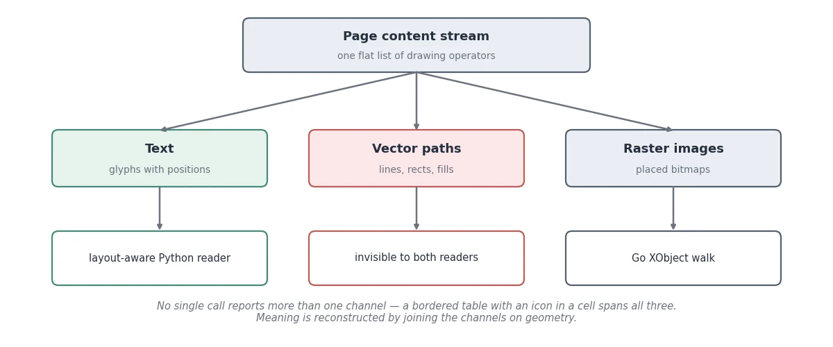A bordered table with a status icon in one cell spans all three channels at once, and no single call returns more than one of them.

There is no unified view because the file has no unified view. You reconstruct meaning by joining the channels on geometry, and that reconstruction is the entire job. Two consequences shape everything downstream:

• A text extractor reads the text channel and nothing else. A chart drawn as vector paths is invisible to it — and so is a chart drawn as a bitmap.
• Any signal of the form “there is content here that the text layer missed” must therefore come from one of the other two channels. That is precisely why a second reader exists.

The two-reader design below covers the text and raster channels. The vector channel is reachable — it takes a third call, and a later section spends real effort on it — but nothing in the pipeline touches it yet, which is what makes vector charts the most durable blind spot in the whole design.

The parser landscape

Four families of tooling exist, and the right policy is a cascade rather than a choice.

Approach	Examples	Where it fits
Classical parsers	pypdf, PyMuPDF, pdfminer.six	Born-digital PDFs with an intact text layer
Commercial extractors	Adobe PDF Extract, Unstructured.io	Complex enterprise document types
OCR	Tesseract, hyperscaler OCR APIs	Scanned pages with no text layer
Vision-language models	Any modern multimodal LLM	Slides, forms, infographics — as a fallback

VLM parsing is the newest and the most tempting. It handles complex layouts that defeat classical parsers. But it is generative: it can hallucinate text, it usually cannot reproduce embedded images, and it is slow and expensive at corpus scale. The sensible policy is cheapest successful parser first — classical parsers, then OCR, then a VLM only for difficult, high-value documents. The rest of this post is that policy made concrete, with a per-page decision that gates the expensive path.

Two readers over the same bytes

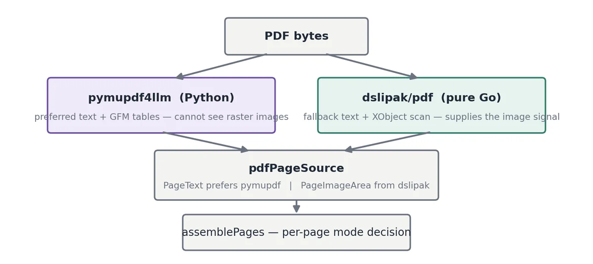
The core architectural move is to run two independent PDF readers over the same file and let each do what only it can do. This is not redundancy — each reader can see something the other structurally cannot.

Both readers converge on one per-page interface. The mode decision downstream needs a signal from each of them.

A layout-aware Python reader such as pymupdf4llm gives you the preferred text: headings recovered from font size and weight, and tables emitted as GitHub-flavoured markdown. What it does not give you is a reliable answer to “is there a big raster image on this page?” A Go PDF library walking Resources → XObject gives you exactly that, plus a flat-text fallback.

The subprocess seam

Most of the practical engineering lives at the Go-to-Python boundary. Spawn the converter once per document, pipe the PDF bytes to stdin, and read back a JSON array of per-page strings so page indices line up with the Go reader’s.

# pymupdf_convert.py - the entire Python side
import sys, json, pymupdf4llm, pymupdf

doc   = pymupdf.open(stream=sys.stdin.buffer.read(), filetype='pdf')
pages = pymupdf4llm.to_markdown(doc, page_chunks=True, header=False, footer=False)
# Page numbers come from the Go side as '## Page N', never from the PDF footer -
# running headers and footers are stripped above.
json.dump([pg['text'] for pg in pages], sys.stdout)

Keeping the Python side this small is what makes the system degrade gracefully. If python3 or the library is missing, the subprocess returns nothing and every page falls through to the Go reader’s flat text. Nothing errors — you simply lose table structure for that run.

Graceful degradation is the right default, but it fails silently. A broken deploy can quietly destroy table quality for weeks with nothing surfacing in the logs. Emit a warning and a metric whenever the fallback path activates, and wrap the spawn in a timeout so one pathological PDF cannot wedge ingestion.

What the structure actually promises

The reader hands back a four-level tree — page, block, line, span — and it is tempting to treat all four levels as facts about the file. Only some of them are.

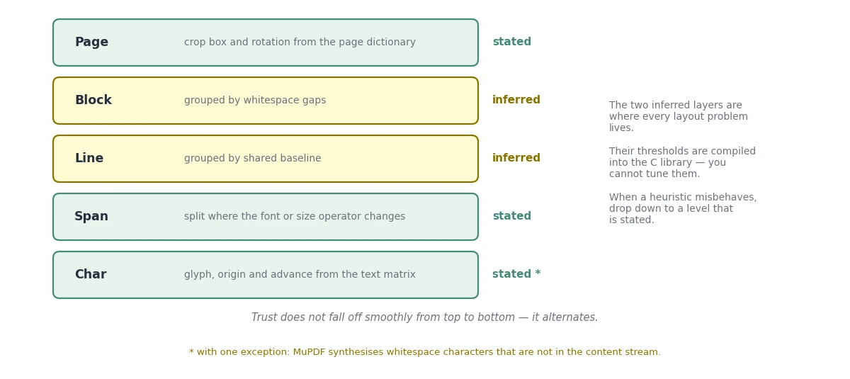Span boundaries and character origins are read off the content stream. Blocks and lines are guesses.

A span ends where the content stream issues a new font or size operator — that boundary is written in the file. Character origins and advances come straight off the text matrix. Blocks and lines are not in the file at all: they are produced by a whitespace-gap heuristic tuned for prose, with thresholds compiled into the C library and no API to reach them.

Notice that trust does not decay smoothly from the top of the tree to the bottom — it alternates. This matters because almost every layout problem lives in those two invented layers: whether a table row arrives as one line or nine, whether a table is one block or twenty. The working rule is to drop down to a level that is stated rather than tune one that is inferred, and it comes up again later when two plausible-looking geometric tests turn out to be broken.

Two normalisations decide whether any later geometric threshold means anything, and PyMuPDF already does both for you — which is precisely why they are easy to break. page.rect is the crop box, already intersected with the media box and translated to the origin. get_text("dict") already returns coordinates in rotated space. The trap is mixing those with values that have not had the same treatment: mediabox, raw content-stream coordinates, or boxes from a second library that puts the origin bottom-left rather than top-left. In particular, do not re-apply the page rotation yourself — on a /Rotate 90 page that inverts every positional test and lands your header band on the side margin, which is the exact bug you were trying to avoid. Nothing throws either way; you simply get plausible wrong answers on the small fraction of pages affected.

When the text layer lies

Before indexing a page you have to answer one question: can this page’s text layer be trusted? Getting this wrong is the most expensive silent failure in the pipeline, because unusable tokens enter the index and stay there.

Why extracted text can be wrong

A PDF stores glyph identifiers — numbers indexing into an embedded, usually subset font — and recovers text through a translation table called the ToUnicode CMap. Subset fonts renumber glyphs in order of first appearance, so glyph 7 might mean c in one document and q in the next. When the CMap is missing or wrong, the extractor still produces output by guessing, and what comes out is typically an arbitrary but internally consistent permutation of the alphabet — a monoalphabetic substitution cipher whose key is unique per font per document.

original:   Unit consumption Rates
extracted:  Vojw dpotvnqujpo Sbuft

Two properties make this the worst kind of failure. Nothing errors — the extractor returns a string, and every layer reports success. And the output looks like text: no replacement characters, just letters. Skimming a log of extracted text, your eye slides right past it.

Why the obvious statistics do not work

A letter swap preserves letter frequencies as a multiset, word lengths, spaces, punctuation and entropy. The classic index-of-coincidence test is exactly invariant under monoalphabetic substitution — permuted English scores like English — so it will confidently certify a corrupted page as clean.

The only property a letter swap destroys is whether the letters spell real words. A lexicon check or a character n-gram model are the only viable instruments. Everything else is permutation-invariant, and therefore blind.

A cascade, not a single ratio

There are five distinct ways a text layer betrays you, and they have different symptoms:

Failure	Cause	Symptom
Broken encoding	Subset font with no ToUnicode CMap	U+FFFD, control runes, private-use codepoints
CID passthrough	Extractor cannot map glyph IDs	Literal (cid:142) sequences
Spacing loss	No space glyphs, or wrong advance widths	Words glued together, or l e t t e r - s p a c e d
Shifted CMap	A wrong but valid mapping	Well-formed Latin letters that spell nothing
Scanned page	No text layer at all	Near-empty string

A bad-rune ratio catches only the first. A scan has no runes at all, and a shifted CMap produces perfectly legal ASCII. So the detector is a cascade of cheap tests, each catching what the others structurally cannot.

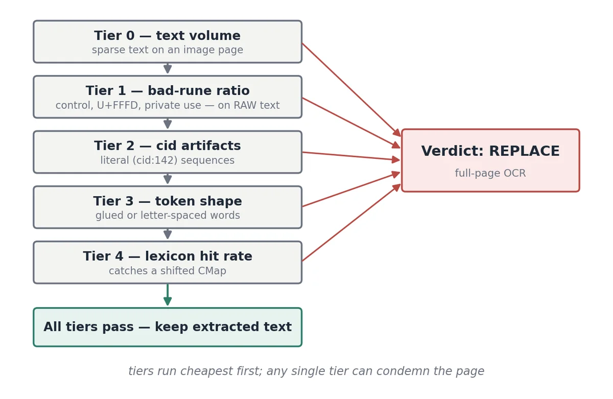Tiers run cheapest first. Four of them can condemn a page outright; the lexicon tier cannot, for a reason that takes until the per-page decision to explain.

// Tier 1: runs on RAW text, before any normalization.
func badRuneRatio(s string) (ratio float64, counted int) {
    var bad int
    for _, r := range s {
        if unicode.IsSpace(r) { continue }   // evidence for neither side
        counted++
        switch {
        case r == utf8.RuneError:            // == '\uFFFD'; also invalid UTF-8
            bad++
        case unicode.IsControl(r):
            bad++
        case unicode.Is(unicode.Co, r):      // private use area
            bad++
        }
    }
    if counted == 0 { return 0, 0 }
    return float64(bad) / float64(counted), counted
}

Ordering gotcha. Compute this ratio on the raw extracted text, before whitespace normalization runs. Normalization scrubs exactly the evidence this tier depends on. Normalize first and the ratio is permanently 0.0, the OCR path never fires, and you index garbage forever with no error anywhere. This deserves an assertion in your test suite, not a comment.

The lexicon tier

This is the tier that catches the shifted-CMap case, and the one most likely to cry wolf on a technical corpus. The check itself is trivial — split into words, look each one up, count the fraction found. Everything difficult is in deciding which tokens are eligible to be judged.

Why it cries wolf	The fix
The page is mostly a table	Score prose blocks only; cells are numbers and codes
Identifiers with digits	Reject any token containing a digit or path character
Short technical tokens	Ignore tokens under four runes (vCPU, EKS, 1x)
Barely any text on the page	Insufficient evidence — assume clean and skip the tier
Domain jargon	Extend the lexicon from your own corpus

Length weighting is the single biggest accuracy win. A four-letter permuted string lands on a real word by accident reasonably often; a nine-letter one essentially never does — the space is roughly 5.4 trillion strings against perhaps forty thousand real words. Weight each token by len - 3 so long tokens carry the evidence, and fail open below a minimum evidence total.

Splitting on !unicode.IsLetter is wrong for identifier-heavy text. Given CEAMVCSRE3110002C it yields CEAMVCSRE — a nine-letter token that misses the lexicon and, under length weighting, misses hard. Split on whitespace first, then reject the whole token if it contains digits.

Building the lexicon

Bigger is not better. Lexicon size trades sensitivity against specificity: a huge word list raises the accidental-hit rate on permuted garbage more than it helps clean pages, which already clear the threshold comfortably. A curated list of roughly twenty thousand common words beats a 300k-word list of inflections and archaisms.

The real gap is domain vocabulary, and the permutation’s own properties give you a nearly perfect harvesting filter:

The substitution key is unique per font per document, so a garbled token such as dpotvnqujpo appears in exactly one document and nowhere else. Real domain vocabulary appears across many. Requiring a candidate to occur in three or more distinct documents filters garbled tokens out almost completely — without ever needing to know which pages were garbled in the first place.

The precondition: what you are allowed to score

The lexicon hit rate answers exactly one question — what fraction of these tokens are real words? — and that question is only meaningful if the tokens were supposed to be words in the first place.

A table cell holding N/A, 14.2, ms or a part number is a correct extraction of correct content, and it misses the word list for reasons that have nothing to do with a broken font. Score it anyway and the page drifts toward the garbled band, not because the detector malfunctioned but because it was asked a question that does not apply to its input.

When two populations you have strong theoretical reason to expect to be separable turn out not to be, suspect the feature extraction before the classifier. Tuning the threshold at that point only changes which mistakes you make.

Derive the gates instead of inventing them. Rather than asking the open-ended question “is this block a table?”, ask a closed one: does this block satisfy the preconditions of the score? Enumerate what the score assumes, then write one cheap test per assumption. The gates stop being a grab-bag of heuristics and become a checklist you can argue about.

The score assumes	Violated by	Cheap test
Running sentences	tables, lists, headings	line count, mean tokens per line
Words made of letters	numeric tables, identifiers, references	letter ratio
A single left margin	grid layouts	distinct line-start positions
No wide gaps inside a line	column gutters	largest intra-line gap
Proportional type	code listings	font name
Body-size type	headings, captions, footnotes	size against the page’s modal size
Text that belongs to the page	running heads, axis labels	position, figure overlap

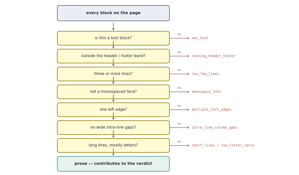Cheapest and most decisive first. The reason codes are not diagnostics — they are how you debug the threshold later.

Combine the gates conjunctively. The two ways of being wrong here are not symmetric:

Error	Consequence	Severity
Excluding genuine prose	The page is judged on the prose that remains; if too much goes, the fail-open rule engages	Mild, self-limiting
Including a table or a code block	The score is computed over input the test does not apply to; the page lands mid-range and the valley narrows corpus-wide	Severe, compounding

Given that asymmetry a block counts as prose only if it passes every gate. The tempting alternative — a weighted score, “looks prose-y on seven of nine axes” — lets a dense table through precisely when it scores well on most axes. Conjunction can only ever shrink the accepted set, which is the direction the asymmetry asks for. Losing a third of your prose blocks to over-eager filtering is fine; letting one dense table through is not.

Fail-open is the other half of the same decision. A conjunctive filter tightened aggressively will empty some pages entirely. The rule that an empty page passes un-scored caps the downside: it converts “I filtered too hard” from a wrong answer into a declined answer. The two choices are a pair — you can only afford to be this conservative because fail-open catches the tail.

This is a scope filter, not a quality filter. Excluding tables from the scorer is not the same as excluding them from the index. Tables are frequently the most valuable content in a technical document, and they are still extracted, chunked, embedded and retrievable. The rule is narrower than it sounds: they do not get a vote on whether the page’s text can be trusted.

Two gates that look right and are not

The two geometric gates are the ones most likely to be wrong in a way you never notice. Both are usually written from an assumption about what the extractor returns, so it is worth measuring that instead of assuming it. The numbers below come from PyMuPDF 1.28 on a synthetic three-cell row — one font, one size, one baseline — with the gutter widened step by step.

MuPDF never leaves a gap. This is the finding that invalidates the obvious implementation. A wide gutter does not come back as empty space between two boxes; MuPDF synthesises a whitespace character whose advance is exactly the width of the gutter. So the natural check — walk adjacent spans, flag next.x0 - prev.x1 above some limit — measures 0.00pt, every time, on every row. Dropping to rawdict and comparing character boxes does not rescue it either: the synthetic space is itself a character, and the between-box gaps are still 0.00pt.

That is also the one exception to the stated-versus-inferred table above. Characters are otherwise read straight off the content stream, but these particular ones are manufactured by the extractor to represent displacement — and they are exactly the characters this gate depends on.

What you get back instead depends on how wide the gutter is, and the boundary is sharp:

Gutter between cells	What the extractor returns	Which gate can see it
below one word space	one line, one span, ordinary spaces	neither — and rightly so
one word space up to 0.80 em	one line, cells in their own spans, gutter carried as an over-wide whitespace character	whitespace width
above 0.80 em	the row is split into separate lines, one per cell	left-edge clustering

The split threshold is a fraction of the font size, and it is emphatically not a multiple of the space width — a distinction that is invisible if you only ever measure one font:

Face	Space advance	Split threshold
Helvetica	0.278 em	0.80 em = 2.9 spaces
Times	0.250 em	0.80 em = 3.2 spaces
Courier	0.600 em	0.80 em = 1.3 spaces

0.80 em held to within a couple of percent across all three faces at 9, 11 and 14pt. It also reproduces on a hand-built PDF whose row is a single TJ operator with kerning offsets rather than separate text-placement calls — 0.79 em stays one line, 0.81 em splits into three — so it is a property of the line-assembly heuristic, not of how the producer happened to emit the row. It is still a property of the library version rather than of the format, so measure it on yours rather than inheriting the number — but measure it in em.

So the gate you want is the advance width of the whitespace character, scaled to the font’s own space and clamped below the split:

def has_column_gap(line, space_advance, size, factor=1.5, split_em=0.80):
    """Wide gutters survive as over-wide whitespace characters, not as gaps.

    space_advance is the font's own advance for U+0020 at this size, via
    pymupdf.Font(fontname=...).glyph_advance(32) * size.

    The clamp is not cosmetic. A gutter wider than split_em never reaches this
    function -- MuPDF has already broken the row into separate lines and
    left-edge clustering owns it -- so the limit must sit strictly BELOW the
    split, or the gate can never fire at all. The 6% headroom below split_em is
    what remains of the usable band once that constraint is satisfied.
    """
    limit = min(factor * space_advance, 0.94 * split_em * size)
    for span in line["spans"]:                 # rawdict: spans carry chars
        for ch in span["chars"]:
            if ch["c"].isspace() and ch["bbox"][2] - ch["bbox"][0] > limit:
                return True
    return False

Monospace is precisely the case a space-relative threshold gets wrong. Courier’s word space is 0.60 em and the split lands at 0.80 em, so the entire band in which this gate can fire is 0.60 to 0.80 em — and a bare factor = 1.5 sits outside it, making the check unfireable on the font family you would most expect to need it for. On a monospaced face the gate is close to useless. That is tolerable here only because the cascade rejects monospaced blocks two gates earlier; reuse this check outside that cascade and the clamp is doing all the work.

The two gates are complementary, and the crossover is that same 0.80 em. Below it the row stays one line and only the whitespace check can fire; above it the row is split and only left-edge clustering can. Neither gate is redundant, and a cascade missing either one has a blind spot sitting entirely on one side of the boundary.

That also sharpens the standing criticism of left-edge clustering. It is often described as the table detector, but it only ever sees tables whose gutters exceed 0.80 em — it is scoring a segmentation decision made upstream by a threshold you cannot reach, and tight-set tables are invisible to it by construction.

Justified prose stretches word spaces by roughly 1.5–2×, which lands inside the band where this check fires — and it does fire: a line set with 1.9× word spaces trips factor = 1.5 just as reliably as a real table row does. That is the “rivers” effect, and it is the reason this gate cannot stand alone. Pair it with vertical consistency, because a genuine column boundary recurs at the same x across many lines and a river does not.

Two smaller corrections worth making at the same time. Scale the clustering tolerance to the block’s modal font size rather than hard-coding points, or the gate behaves differently on a 9pt journal and a 14pt report. And take that mode weighted by characters, not by span count — several short bold runs will otherwise outvote the body text.

One more precondition: reading order

The score is computed over joined text. If the page is two-column and the blocks are concatenated in the wrong order, you are scoring a string that never existed on the page. Every word in it is real, so the lexicon tier passes it happily and the damage surfaces much later, as chunks that read as non-sequiturs while being perfectly well-formed.

Sorting blocks by (y, x) is the obvious fix and is exactly wrong for two columns — it walks across the page line by line, alternating between them. Detect gutters instead: project every text block onto the x-axis and look for an interior vertical strip that no text crosses, wider than about 8pt. Discard runs touching the page edges, which are margins rather than gutters. Then order column-major.

You can check your own work without labels. Count broken seams — a block ending without terminal punctuation followed by a block starting with a capital, which means a sentence was cut and its continuation jumped elsewhere. Try the extractor’s native order, a naive (y, x) sort and column-major ordering, and keep whichever produces the fewest. On a single-column page all three agree, so it degrades gracefully.

Calibrating the threshold

This tier earns its complexity because the two populations separate unusually well. Permuted text does not score somewhat lower than English; it scores near zero.

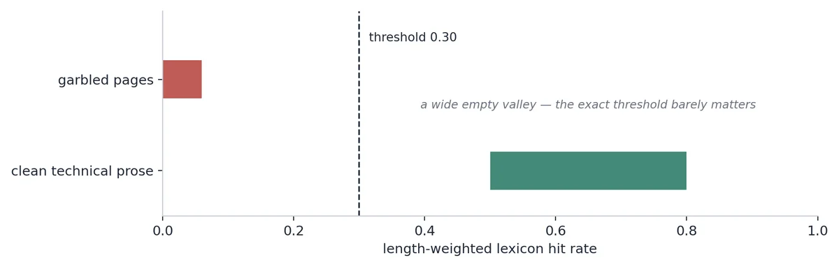When the threshold sits in a wide empty valley, its exact value barely matters.

Expect clean technical prose to land lower than general English — roughly 0.50–0.80 with a 20k-word lexicon, against 0.80+ for a novel. That gap is domain vocabulary, which is why the harvest step matters.

It is worth being clear about where that empty stretch comes from, because it is easy to assume it is a property of a well-built detector:

A valley is a property of the failure mode, not of the classifier. A font’s character map is either right or wrong — there is no partial setting, so no mechanism produces a page halfway between. Graded failures produce no valley at all, however good your detector is. Before building any threshold detector, ask which kind of failure you have.

Do not guess thresholds. Dump per-page signals as JSONL during ingestion, histogram them over a few hundred real pages, and look for the valley. And you never need to find garbled PDFs to test with: manufacture perfectly labelled data by applying the same transformation the broken font applies. Shuffle the alphabet with a seeded RNG, leave digits, punctuation and whitespace untouched — that is faithful to the real failure. Garble a hundred clean pages with a few fixed seeds and assert in CI that every clean page scores above threshold and every garbled variant below.

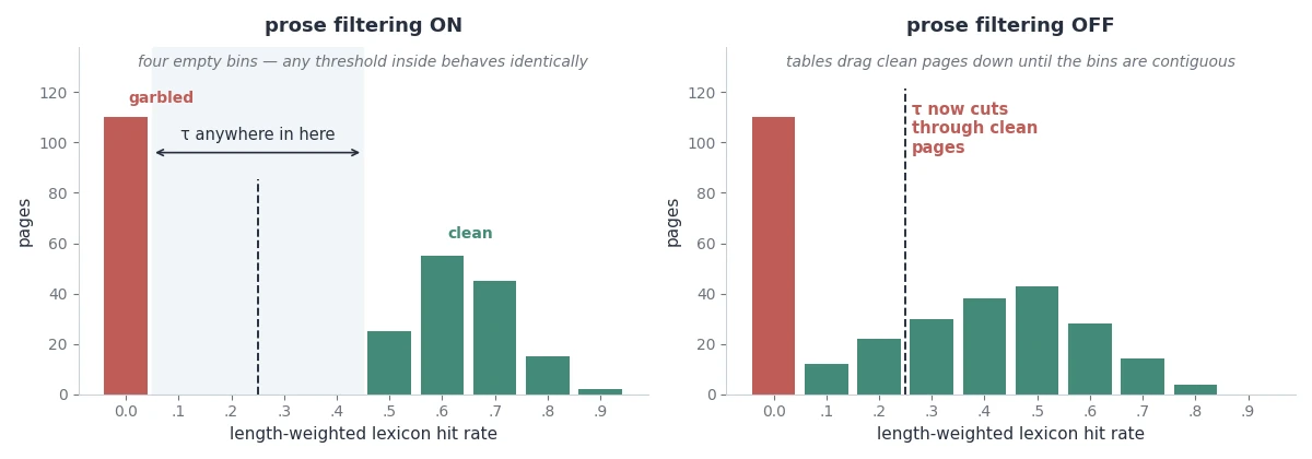The prose filter is what creates the valley. Calibration only locates it.

Which statistic finds the valley

The obvious method is the widest gap between adjacent sorted scores. That is a fine way to place the threshold once a valley exists, and its refusal condition is genuinely useful — if the widest gap is under about 0.2, raise an error rather than returning a plausible-looking number. A narrow gap means the two populations touch, and by far the most common reason is non-prose leaking into the token stream; the next section works through the others. Either way the bug is upstream, and no threshold will save you.

It is a poor statistic for comparing runs, though, and comparing runs is exactly what you want while tuning the prose filter. The maximum of adjacent differences is an extreme order statistic dominated by wherever your data happens to be sparse; one outlier moves it, so “did the gap widen?” is a noisy question to ask of a change. Otsu’s between-class variance uses every observation and hands you the threshold as a by-product — one pass over the sorted scores:

def separability(scores, n_pages, min_coverage=0.7):
    """Otsu between-class variance over an unlabelled score column.

    Returns (J, threshold). Every observation contributes, which makes this
    stable enough to compare across runs -- the widest-gap statistic is not.

    n_pages is the page count BEFORE prose filtering and fail-open dropped
    anything. The coverage floor is not optional: J is maximised by BALANCED
    classes, so without it the cheapest way to raise the objective is to
    filter until fifteen pages survive and happen to split 8/7.
    """
    s = sorted(scores)
    n = len(s)
    if n < 30 or n < min_coverage * n_pages:
        return 0.0, None

    total, run, best = sum(s), 0.0, (0.0, None)
    for t in range(1, n):
        run += s[t - 1]
        w0 = t / n
        j = w0 * (1.0 - w0) * (run / t - (total - run) / (n - t)) ** 2
        if j > best[0]:
            best = (j, s[t])
    return best

Use the gap width for the go/no-go and for the margin you graph over time. Use Otsu as the objective when you are asking whether a change to the prose filter helped. With the coverage floor in place, a change that raises it is an improvement and one that lowers it is a regression — you are measuring the thing you care about rather than a proxy for it, which is rare enough in classifier work to exploit when it is available.

Any label-free objective is an invitation to an optimiser, and an optimiser will find the cheat before you do. Coverage is the obvious one; the other is a minimum character count per scored page, because a page reduced to one eight-word sentence produces a high-variance score that lands anywhere. Guard both before you trust a search over the prose-filter parameters.

What the valley actually buys, and when it does not

Two facts get bundled together here, and only one of them is free.

The first is unconditional. Both error counts are step functions of the threshold: they change only at the score of an observed page, so between two adjacent data points every threshold is the same classifier, byte for byte. That holds for any data at all, and it means only a couple of hundred candidate thresholds ever need checking rather than a continuum.

The second is a property of your corpus — that a threshold exists where both counts are zero. That happens exactly when the lowest-scoring clean page still outscores the highest-scoring garbled page. When it holds, expected cost is zero for any relative cost of the two error types, and the cost ratio you would otherwise have to estimate and defend in review drops out of the problem entirely. When it fails, you are doing ordinary classifier work whether you like it or not.

So check it rather than assuming it. The cheapest sufficient test is that no (clean, garbled) pair sits in the wrong order. Counting those pairs is far more robust than comparing the two extremes, because a single mislabelled page destroys the extremes and barely moves the count:

from bisect import bisect_left

def inversions(clean, garbled):
    """Pairs sitting in the wrong order. Zero is exactly separability."""
    g = sorted(garbled)
    return sum(len(g) - bisect_left(g, c) for c in clean)

def separated_pairs(clean, garbled):
    """Exactly 1.0 is the licence to treat the threshold as free.

    This is ROC area with ties counted against you rather than at a half.
    That is deliberate: a tie means a clean and a garbled page scored
    identically, and no threshold can separate identical scores. Textbook AUC
    would report 1.0 there, in a case where no zero-error threshold exists.
    """
    n = len(clean) * len(garbled)
    return 1.0 - inversions(clean, garbled) / n if n else 0.0

If they do overlap, work the causes in order and do not skip to the last one:

1. Assume the feature is wrong before the world is. Tables leaking past the prose gate push clean pages down. A vocabulary harvest run without the three-document filter pushes garbled pages up. Unsupported-language pages pile up in the middle. Each has a distinct fingerprint in the reason-code histogram, and every one of them is a measurement defect that tuning cannot fix.
2. Segment before you tune. Mixing born-digital pages with pages someone already OCR’d puts two different physical failures on one axis. Split them and one class often shows a clean valley while the other never will — which tells you which one needs expensive treatment and lets the other keep its free threshold.
3. Add a dimension. Overlap in one projection is not overlap in the data. Populations that interleave on the lexicon axis frequently separate cleanly in the plane once you add trigram similarity or evidence. This is the reason to log signals that nothing consumes yet: they are cheap to write and impossible to backfill.
4. Only then, accept it and abstain. Two thresholds with an uncertain band between them converts an unavoidable error into a bounded cost. Watch the fraction of the corpus that lands in the band rather than its width — under 5% is a healthy safety valve, over 30% and the band is doing the classifying, which means going back to step 3.

Partial corruption hides inside a page average

Everything so far scores a page. That turns out to be the wrong unit, and the reason is arithmetic rather than anything to do with PDFs.

Suppose a fraction $\alpha$ of a page extracted cleanly and the rest is garbage — where $\alpha$ is the share of length-weighted token mass, since that is the denominator the hit rate actually divides by. The lexicon hit rate is a weighted mean over tokens, so the page’s score is simply the clean rate scaled by $\alpha$: a straight line. With clean technical prose sitting around 0.65 and τ at 0.30, that line does not reach the threshold until 54% of the page is gone.

The trigram tier that the language check relies on is worse rather than better. Junk trigrams land in slots the language rarely uses, so the clean and junk profiles are close to orthogonal and the similarity follows a curve instead of a line:

\[\cos \;=\; \frac{\alpha}{\sqrt{\alpha^{2} + (1-\alpha)^{2}}}\]

On that measure a page 30% destroyed still scores 0.92.

That curve assumes the two profiles have similar concentration. Real junk is flatter — higher entropy, and therefore a smaller norm once normalised — which pulls the measured cosine somewhat below the curve. Treat it as the shape of the problem rather than a calibration you can invert to recover $\alpha$.

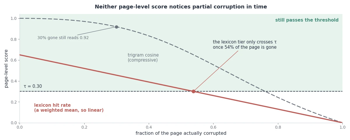Neither score reaches the threshold until the page is more than half gone.

Neither score is broken. Both are averages, and an average over a page cannot localise damage that occupies only part of a page. Partial corruption is therefore not merely hard to detect at page level — it reads as clean right up to the point where the page is past saving anyway.

The fix is to change the denominator, not the threshold. Partition the text by font and score each font separately, because that matches the physical failure: one embedded font loses its character map and every character drawn in it is garbage wherever it happens to sit on the page, while text in the other fonts is untouched.

def corrupted_fraction(prose_blocks, lexicon, floor=0.30, min_evidence=40.0):
    """Share of judgeable characters drawn in a font that scores as garbled.

    Takes prose blocks only -- the precondition that governs the page-level
    score governs the per-font score in exactly the same way. Reuses the
    lexicon tier, so it needs no machinery the pipeline does not already have.
    """
    buckets = {}
    for block in prose_blocks:
        for line in block.lines:
            for span in line.spans:
                buckets.setdefault(span.font, []).append(span.text)

    judged = bad = abstained = 0
    per_font = {}
    for font, chunks in buckets.items():
        text = " ".join(chunks)
        score, evidence = lexical_score(lexical_tokens(text), lexicon)
        if evidence < min_evidence:
            per_font[font] = None            # abstain -- NOT counted as clean
            abstained += len(text)
            continue
        per_font[font] = score
        judged += len(text)
        if score < floor:
            bad += len(text)

    total = judged + abstained
    return (bad / judged if judged else 0.0,
            abstained / total if total else 0.0,
            per_font)

Report the abstained share beside the ratio and never fold it into the denominator. A font carrying six words of italics has no usable evidence, and quietly counting its characters as clean is the same dilution this section exists to warn about, one level further down.

That gives you three things for the price of one: a corrupted fraction that is a genuine character ratio over text you could actually judge, the identity of the broken font, and that font’s text isolated — which is exactly the input the repair step needs. Run the page-level score as a cheap screen and pay for the per-font pass only on the pages that fail it.

The font is the unit of everything

Once you notice that the corruption is scoped to a font rather than a page, the same fact keeps paying out. It gives you the near-zero score, the perfectly labelled synthetic data, the label-free vocabulary harvest, and two more things that are easy to miss.

Pages that cannot judge themselves can borrow a verdict. Conservative prose filtering opens a hole: a page that is entirely table — a spec sheet, an appendix — has every block excluded, no evidence at all, and fails open to TEXT. If that table was garbled you have just indexed nonsense with no signal anywhere. But if ABCDEF+MinionPro produced garbled prose on pages 3, 7 and 12, then every block using that font in that document is garbled, including the table on page 40 that has no prose of its own.

// Valid only because the corruption is font-scoped and deterministic --
// the same property the vocabulary harvest relies on.
type fontEvidence struct {
    bad   map[string]float64
    total map[string]float64
}

func (f *fontEvidence) observe(font string, weight float64, gibberish bool) {
    f.total[font] += weight
    if gibberish {
        f.bad[font] += weight
    }
}

func (f *fontEvidence) garbled(font string, minEvidence float64) bool {
    total := f.total[font]
    if total < minEvidence {
        return false // not enough to say either way; do not guess
    }
    return f.bad[font]/total > 0.5
}

This needs a second pass over the document, which you already need for header and footer detection — repetition is only visible across pages. Fold the two together.

Repair is often cheaper than re-OCR. REPLACE is not the only possible response to a broken font. The corruption is a bijection on the alphabet, which means it is invertible, and the character-trigram profile identifies which bijection.

Subset fonts assign glyph IDs in the original font’s order, so for a subset of an ordinary text font the letters usually keep their relative order and what you get is the true text plus a constant offset. Sweep the candidate offsets, rebuild the profile for each, and score it against your language references:

def recover_shift(text, reference):
    """Find the rotation that turns junk back into language.

    One candidate spikes into the clean band and the rest sit near zero, so
    the profile certifies its own answer -- no labels needed. When the offset
    lives in glyph-ID space rather than the alphabet, sweep the codepoint
    offset over a few hundred candidates instead of 26.
    """
    best = (0.0, 0, text)
    for k in range(1, 26):
        candidate = "".join(
            chr((ord(c) - 97 - k) % 26 + 97) if "a" <= c <= "z" else c
            for c in text.lower()
        )
        score = cosine(profile(candidate), reference)
        if score > best[0]:
            best = (score, k, candidate)
    return best

Two things make this far easier than classical cryptanalysis. Word spaces usually survive, because gaps come from positional moves in the content stream rather than from a space glyph — so the boundary trigrams, the most discriminative features any language has, snap into alignment the moment the offset is right. And the mapping is per font, not per page: solve it once, cache it, and fix every page in the document that uses that font.

Arbitrary permutations need hill-climbing — start from a frequency-matched key, swap two symbols, keep the swap when the trigram score improves — and converge on a few hundred characters of English. Some cases are genuinely unrecoverable: many-to-one mappings have destroyed information, ligatures break the one-to-one assumption, and CJK has too large a symbol set with too little text per page. In all three the score simply fails to climb, which is itself the answer.

Accept a repair only when the recovered text scores inside the clean band, and fall through to OCR otherwise. A repaired page costs a few milliseconds of CPU; an OCR’d page costs a vision call and comes back with graded errors of its own. Where repair works it is strictly better — and it works on exactly the failure this whole section is about.

The per-page decision

Three signals — the gibberish verdict, the language verdict and the figure area — classify each page into one of four modes. The two additions are not refinements; each closes a hole that would otherwise burn money silently.

The language blind spot

A French page scored against an English lexicon lands at 0.05–0.15 — the same band as garbled text. The classifier is answering the question it was asked, and the question was wrong.

The consequence is worse than a misclassification. REPLACE means discard the text and OCR the page. OCR the French page and you get back French text, which scores just as low. You have spent a vision call to arrive exactly where you started — and if anything in the pipeline retries on failure, you have built a loop that bills by the page.

The signal that separates them falls out of what a substitution cipher does. It maps every trigram to some other trigram, so English’s the, ing and ion become strings that match no natural language, because the relabelling is a random key. Real French is dense in real French trigrams. So build character-trigram profiles per language and take the best match — scoring low against every profile is a signature no real language produces.

Text	vs English	vs French	vs German
clean English	0.91	0.46	0.41
clean French	0.44	0.89	0.43
garbled English	0.07	0.06	0.05

Trigrams are the right window size. Single characters are too weak — a permutation preserves the shape of the letter-frequency curve, so frequency tests certify garbled pages as clean. Four- and five-grams discriminate better but the space grows exponentially and needs far more text per page to estimate stably.

This tier inherits the same precondition as the lexicon tier, and more sharply. Fold every non-letter to a space and a table of part numbers collapses to a single space — no trigrams, an empty profile, and a similarity of exactly 0.0. A perfectly extracted numeric table scores identically to total corruption. Because this tier is what distinguishes “unsupported language” from “garbled”, a table leaking through here does not merely dilute a score: it confidently routes a clean page to OCR.

A page that scores low on the lexicon but matches a language profile strongly therefore needs a mode of its own, alongside TEXT, FIGURES and REPLACE. Call it LANG: keep the extracted text, because it is correct and merely unjudgeable, tag it with the detected language so retrieval can filter on it, and record the gap so it stays visible.

LANG has to be a terminal mode, not an error path. If it falls through to the OCR branch you have rebuilt the loop this section exists to prevent — OCR returns the same unsupported language, it scores the same, and any retry-on-failure logic will do it again.

Counting LANG pages per language tells you which lexicon to add next, so the metric doubles as the roadmap. And decide the language once per document from concatenated text rather than per page — identification from 200 characters is genuinely uncertain, from 2000 it is nearly perfect.

Vector figures are invisible to a raster signal

The image signal is raster-only by construction: the Go reader walks Resources → XObject, and a chart from matplotlib, D3, Illustrator or Visio contains no XObject at all. It is path-fill and path-stroke operators — the middle channel, which neither reader reads.

So the page reports zero image area, zero gibberish, and lands in TEXT. The chart’s meaning is discarded and its tick labels are indexed as free-floating numbers, which is worse than nothing because they pollute retrieval.

Detecting it means classifying paths before counting them, since pages are full of paths that are not figures — table rules, underlines, borders, bullets:

def is_furniture(path, page_area):
    """Table rules, underlines, borders, hairlines and tiny marks."""
    r = path["rect"]
    w, h = r.x1 - r.x0, r.y1 - r.y0
    if w * h < 0.0002 * page_area:
        return True                                   # bullet, tick, dot
    if min(w, h) <= 2.0 and max(w, h) > 20.0:
        return True                                   # a rule or underline
    return path.get("fill") is None and path.get("stroke_opacity", 1) == 0

Cluster what survives, then require at least one curve or diagonal segment in the cluster: charts have them and a grid of boxes does not. Two traps are worth knowing in advance. Some producers draw a full-page white background rectangle — one path, huge area, no curves — which the curve requirement handles. Others draw text as outlines, one path per glyph, producing thousands of small curved paths that look exactly like a figure; guard against that by checking whether the cluster also overlaps substantial extracted text.

Text blocks sitting mostly inside a detected figure region are axis labels and legends. They are not prose, and excluding them closes the loop back to the prose gate.

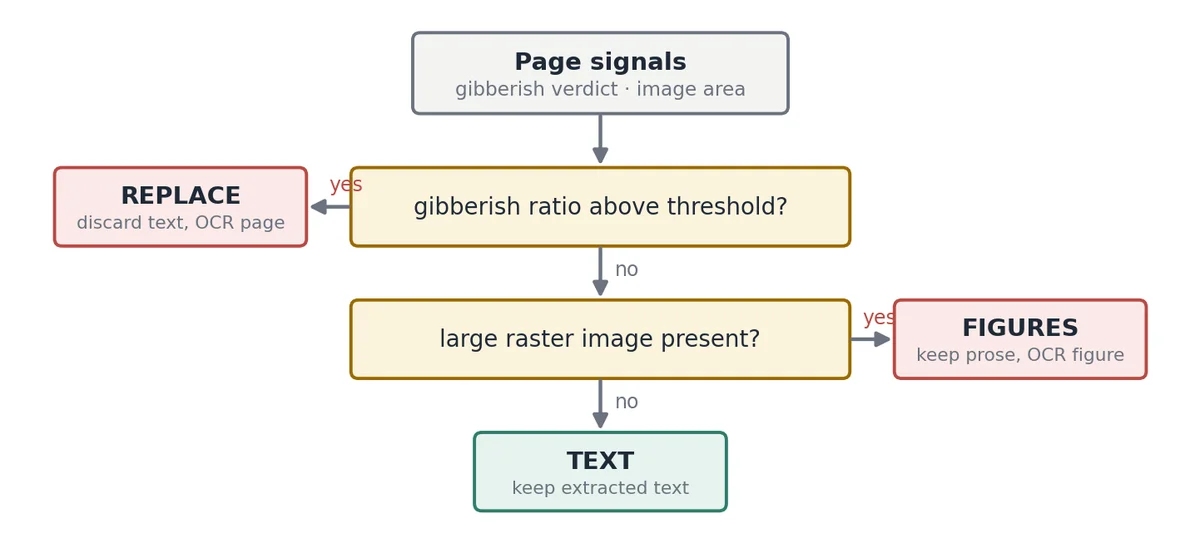The expensive vision path is gated behind this decision, so you pay vision rates only on pages that need them.

FIGURES mode is where the two readers combine on a single page, and it is the scenario the design was tuned for. On a pricing page, the Python reader extracts the surrounding prose cleanly, but the actual rate numbers are baked into a large raster image it cannot read. The Go reader reports the image, FIGURES fires, and the output carries both: clean prose under ## Page N, plus a figures-only transcription appended under ## Page N (transcribed figures). REPLACE is the harsher relative — when the text layer itself is garbage, OCR replaces the whole page.

Three refinements are worth building in from the start:

• Tier 0 is asymmetric. No text and no image is a genuinely blank page, and OCR would spend a vision call to produce nothing. No text with a big image is a scan. Same ratio, opposite action — the second reader’s image signal disambiguates.
• Add a document-level prior. If more than ~60% of a document’s pages landed in REPLACE, it is a scan throughout; promote the borderline pages too. Documents are homogeneous, and a page-independent classifier throws that information away.
• Persist the decision. Store the mode, the signal values and an extractor_version per page. Re-ingestion becomes idempotent, decisions are auditable months later, and a threshold change tells you exactly which documents need re-extraction.

The cost asymmetry should drive where you put the thresholds. A false positive — a clean page sent to OCR — costs one vision call and slightly worse text. Loud and bounded. A false negative — a garbled page indexed as clean — puts unsearchable tokens in the keyword index and a meaningless vector in the vector index. Silent, permanent, and degrading every query that should have hit that page.

Classify provenance before you trust any threshold

One more split has to happen before the numbers above mean anything, and it is easy to miss because it only bites on mixed corpora.

Nothing in PDF converts pixels to text. A scanned page has no fonts and no character map, so the failure this post is about cannot occur there at all. What happens instead is that OCR adds a second layer: invisible text — render mode 3, never painted — in a glyphless placeholder font, positioned to match the words in the image, carrying a ToUnicode map that the OCR tool generated itself and which is therefore correct by construction. The scan and the text sit on the same page, and nothing checks that the two layers agree.

	Born-digital	Raw scan	Scanned, then OCR’d
Character map	often wrong	absent	correct by construction
Extraction yields	real text or cipher nonsense	empty string	the engine’s best guess
Characteristic failure	substitution cipher	nothing extractable	graded misreadings
Score behaviour	near 1.0 or near 0.0	no evidence	anywhere in between

That last row is the problem. OCR errors are graded — 3% character error leaves most long words intact, 15% leaves few — so OCR’d pages land smoothly across the middle of the score axis and fill the valley. It looks exactly like a broken prose filter, but the preprocessing is fine. You are scoring two different physical failures on one axis.

So classify provenance first, then route. A page with no text and a full-page image is a raw scan. A page whose font list includes a glyphless placeholder, or which carries invisible text over a large image, is an OCR sandwich — judge it with the engine’s own confidence if you have it, or with a separate threshold, and never with the born-digital one. Engine confidence is the better signal where available, because it is calibrated to actual uncertainty rather than inferred from it.

Three failure modes belong to the sandwich alone and are worth a check each: double OCR, where a page that already had a text layer gets another one and extraction returns every word twice; OCR in the wrong language, which produces confident, plausible, wrong words that are genuinely hard to tell from garbling; and systematic confusions such as rn→m, l→1 and cl→d, which are stable per font and scan quality and therefore cluster rather than scatter. A miss rate that stays suspiciously constant across a document is the tell.

What the text cascade structurally cannot see

Everything so far asks whether the characters are wrong. A different failure is that they are absent — extraction returned materially less than the page visibly carries. An empty string and a genuinely short page look identical to code that only checks whether extraction succeeded.

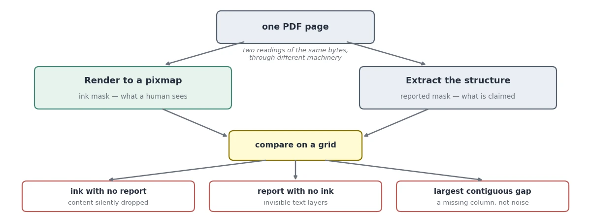Where the two readings agree, extraction is faithful. Where they disagree, the rasteriser is the one to believe.

Render the page to a low-resolution greyscale pixmap and threshold it into an ink mask — what a human would see. Separately paint the bounding boxes the extractor reported — text spans, image placements, vector paths — onto the same grid. The independence is the whole asset: glyph rendering and glyph-to-Unicode mapping are separate concerns in every PDF engine, so a font can draw perfectly while carrying no usable character map. And when they disagree, the rasteriser is the more trustworthy of the two, because its output is by definition what a human sees.

import numpy as np
import pymupdf

def ink_mask(page, dpi=72, dark=0.75):
    """Boolean mask of what is actually visible on the page."""
    pix = page.get_pixmap(dpi=dpi, colorspace=pymupdf.csGRAY, alpha=False)
    a = np.frombuffer(pix.samples, dtype=np.uint8).reshape(pix.height, pix.width)
    background = np.percentile(a, 90)      # never assume the page is white
    return a < background * dark

Five details matter more than they look:

• 72 dpi is plenty, and roughly sixteen times cheaper than 300.
• Do not assume a white background. Estimate it from a high percentile of the histogram, or every scan with a grey cast reads as solid ink.
• Paint span boxes, not block boxes. A block box swallows the inter-line whitespace and hides exactly the gaps you are looking for.
• Pool the grid with any, not a mean. Averaging dilutes a cell holding one thin line of text below any sensible threshold.
• The signal is the largest contiguous region of unreported ink, not the total. Scattered disagreement is anti-aliasing; a contiguous block is a missing column.

Characters per unit ink is a tempting cheap substitute, and it fails on exactly the pages you care about: a page that is one large chart has high ink and almost no characters — the same coordinates as a scan. Unreported ink separates them, because the chart is reported, as an image block.

Rendering and reconciling together cost on the order of 50ms a page, so gate them. Character count, font metadata, replacement-character rate and the page’s deviation from its own document’s median are all effectively free, and only pages failing one of them should pay for a pixmap. That two-stage shape — cheap gate, then an expensive confirming pass on the minority that fail it — is the same one that governs page-level versus per-font scoring.

Prefer a within-document baseline to a corpus-wide constant wherever you can. Characters per unit ink varies enormously between Latin, CJK and mathematics, and watermarks inflate ink uniformly across a document. A constant has to be retuned for every document type you onboard; a baseline computed fresh from the document absorbs all of it for free.

One limit worth stating plainly: both channels can fail together on a damaged or encrypted page, so the absence of disagreement is not evidence of health. Make render-success a separate gate, and never let a page that failed to parse be silently dropped — quarantine it where someone will see it.

The inverse case: text with no ink

Reconciliation hunts for ink the extractor never reported. The mirror failure is text the extractor does report that was never rendered at all, and nothing above can see it — every statistic in this post assumes the characters were meant to be read. Extractors will happily lift text drawn white-on-white, at 0.1pt, with an alpha of zero, positioned outside the crop box, or in render mode 3 — the OCR sandwich above, seen from the other side.

That overlap is the reason this check reports rather than drops: the sandwich is legitimate and common, so a rule that deleted every invisible span would delete the text layer of every OCR’d page in the corpus. What is left once you exclude it is the interesting part, because nothing else legitimately hides text — which is why the same signals become a security filter the moment the corpus is untrusted, as part 8 picks up.

Everything you need is already in the span dictionary you are walking: size below about 4pt, an alpha of zero, a degenerate or off-cropbox bbox, and the span’s color against the fill rect painted beneath it — under roughly 0.06 luminance difference nobody can read it. Run it in report mode first and tune the thresholds against your own corpus before it drops anything. Two caveats: alpha is absent on older PyMuPDF builds, and crop-box comparison needs page rotation normalised first.

Three table representations, deliberately

How a table gets extracted depends entirely on where it came from, and it is worth keeping three renderings rather than forcing one:

Source	Extractor	Output shape
.xlsx / .csv file	Direct linearization	Header: value | Header: value rows
Born-digital PDF	Layout-aware parser	GFM pipe table
Raster image or garbled font	Vision OCR	Header: value rows, by prompt design

Normalising these into one schema means re-parsing structure you have either already lost or already have. Keeping extraction and chunking decoupled through plain text, rather than a shared typed schema, is precisely what lets the OCR path participate at all, since a vision model produces prose and nothing else.

The chain in one pass

A PDF stores glyph codes, not characters, and the map back is optional and frequently wrong. That failure is silent, font-scoped, deterministic and structure-preserving — in other words, a substitution cipher on the alphabet.

A cipher destroys word identity completely, because real words are vanishingly sparse in string space. So the fraction of tokens that are real words separates the two cases by orders of magnitude rather than by degree, which is what produces an empty valley in the score distribution. Inside that valley both error counts are zero, so expected cost is zero for any cost ratio and the hardest judgement call in threshold-setting evaporates — provided you check that the valley is really there rather than assuming it.

The valley narrows when domain vocabulary is missing, which is what harvesting fixes. It closes when non-prose leaks into the token stream, which is what the prose gate prevents — or when two provenances get scored on one axis, which is what provenance classification prevents. And because the corruption belongs to a font rather than a page, the same single fact hands you the labelled test data, the label-free vocabulary harvest, the verdict for pages with no judgeable text, and the key needed to repair the text without OCR at all.

If you track one number from this entire post, track the margin between the lowest-scoring clean page and the highest-scoring garbled one, on every CI run. The binary assertion only fires once the valley has already closed, by which point you are debugging a production incident. The margin turns that cliff into a gradient you can watch erode over months.

What comes next

The chunker in the next post does not care which of the three representations it receives — it recognises “this is a table” from the text itself.

References

1. Ofer Mendelevitch and Forrest Sheng Bao, Hands-On RAG for Production, O’Reilly Media, 2026
2. PyMuPDF and pymupdf4llm documentation
3. Tesseract OCR
4. PDF 32000-1:2008 — Document management, Portable Document Format
5. Nobuyuki Otsu, “A Threshold Selection Method from Gray-Level Histograms”, IEEE Transactions on Systems, Man, and Cybernetics, 1979
6. William B. Cavnar and John M. Trenkle, “N-Gram-Based Text Categorization”, SDAIR, 1994